Artificial Intelligence Certification Course
- 19k Enrolled Learners
- Weekend
- Live Class
In the era of Machine Learning and Deep Learning, Restricted Boltzmann Machine algorithm plays an important role in dimensionality reduction, classification, regression and many more which is used for feature selection and feature extraction. This Restricted Boltzmann Machine Tutorial will provide you with a complete insight into RBMs in the following sequence:
This Edureka video on “Restricted Boltzmann Machine” will provide you with a detailed and comprehensive knowledge of Restricted Boltzmann Machines, also known as RBM.
Let’s begin our Restricted Boltzmann Machine Tutorial with the most basic and fundamental question,
What are Restricted Boltzmann Machines?
Restricted Boltzmann Machine is an undirected graphical model that plays a major role in Deep Learning Framework in recent times. It was initially introduced as Harmonium by Paul Smolensky in 1986 and it gained big popularity in recent years in the context of the Netflix Prize where Restricted Boltzmann Machines achieved state of the art performance in collaborative filtering and have beaten most of the competition.
It is an algorithm which is useful for dimensionality reduction, classification, regression, collaborative filtering, feature learning, and topic modeling.
Now let’s see how Restricted Boltzmann machine differs from other Autoencoder.
Autoencoder is a simple 3-layer neural network where output units are directly connected back to input units. Typically, the number of hidden units is much less than the number of visible ones. The task of training is to minimize an error or reconstruction, i.e. find the most efficient compact representation for input data.

RBM shares a similar idea, but it uses stochastic units with particular distribution instead of deterministic distribution. The task of training is to find out how these two sets of variables are actually connected to each other.
One aspect that distinguishes RBM from other autoencoders is that it has two biases.
Now that we know what is Restricted Boltzmann Machine and what are the differences between RBM and Autoencoders, let’s continue with our Restricted Boltzmann Machine Tutorial and have a look at their architecture and working.
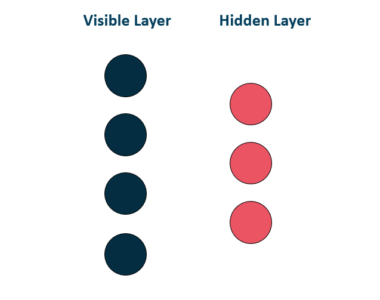
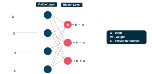
Restricted Boltzmann Machines are shallow, two-layer neural nets that constitute the building blocks of deep-belief networks. The first layer of the RBM is called the visible, or input layer, and the second is the hidden layer. Each circle represents a neuron-like unit called a node. The nodes are connected to each other across layers, but no two nodes of the same layer are linked.
 The restriction in a Restricted Boltzmann Machine is that there is no intra-layer communication. Each node is a locus of computation that processes input and begins by making stochastic decisions about whether to transmit that input or not.
Each visible node takes a low-level feature from an item in the dataset to be learned. At node 1 of the hidden layer, x is multiplied by a weight and added to a bias. The result of those two operations is fed into an activation function, which produces the node’s output, or the strength of the signal passing through it, given input x.

Next, let’s look at how several inputs would combine at one hidden node. Each x is multiplied by a separate weight, the products are summed, added to a bias, and again the result is passed through an activation function to produce the node’s output.

At each hidden node, each input x is multiplied by its respective weight w. That is, a single input x would have three weights here, making 12 weights altogether (4 input nodes x 3 hidden nodes). The weights between the two layers will always form a matrix where the rows are equal to the input nodes, and the columns are equal to the output nodes.

Each hidden node receives the four inputs multiplied by their respective weights. The sum of those products is again added to a bias (which forces at least some activations to happen), and the result is passed through the activation algorithm producing one output for each hidden node.
Now that you have an idea about how Restricted Boltzmann Machine works, let’s continue our Restricted Boltzmann Machine Tutorial and have a look at the steps involved in the training of RBM.
Check out this Artificial Intelligence Course with Python training by Edureka to upgrade your AI skills to the next level
The training of the Restricted Boltzmann Machine differs from the training of regular neural networks via stochastic gradient descent.
The Two main Training steps are:
The first part of the training is called Gibbs Sampling. Given an input vector v we use p(h|v)for prediction of the hidden values h. Knowing the hidden values we use p(v|h) :
 for prediction of new input values v. This process is repeated k times. After k iterations, we obtain another input vector v_k which was recreated from original input values v_0.

The update of the weight matrix happens during the Contrastive Divergence step. Vectors v_0 and v_k are used to calculate the activation probabilities for hidden values h_0 and h_k :

The difference between the outer products of those probabilities with input vectors v_0 and v_k results in the updated matrix :
Using the update matrix the new weights can be calculated with gradient ascent, given by:
 Now that you have an idea of what are Restricted Boltzmann Machines and the layers of RBM, let’s move on with our Restricted Boltzmann Machine Tutorial and understand their working with the help of an example.
 RBMs have found applications in dimensionality reduction, classification, collaborative filtering and many more. They can be trained in either supervised or unsupervised ways, depending on the task.
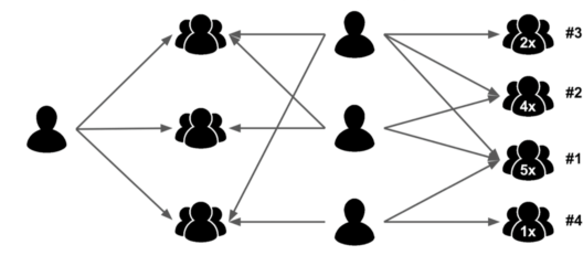
Let us assume that some people were asked to rate a set of movies in the scale of 1-5 and each movie could be explained in terms of a set of latent factors such as drama, fantasy, action and many more. Restricted Boltzmann Machines are used to analyze and find out these underlying factors.

The analysis of hidden factors is performed in a binary way, i.e, the user only tells if they liked (rating 1) a specific movie or not (rating 0) and it represents the inputs for the input/visible layer. Given the inputs, the RMB then tries to discover latent factors in the data that can explain the movie choices and each hidden neuron represents one of the latent factors.
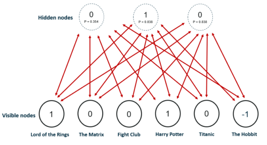
Let us consider the following example where a user likes Lord of the Rings and Harry Potter but does not like The Matrix, Fight Club and Titanic. The Hobbit has not been seen yet so it gets a -1 rating. Given these inputs, the Boltzmann Machine may identify three hidden factors Drama, Fantasy and Science Fiction which correspond to the movie genres.
After the training phase, the goal is to predict a binary rating for the movies that had not been seen yet. Given the training data of a specific user, the network is able to identify the latent factors based on the user’s preference and sample from Bernoulli distribution can be used to find out which of the visible neurons now become active.

The image shows the new ratings after using the hidden neuron values for the inference. The network identified Fantasy as the preferred movie genre and rated The Hobbit as a movie the user would like.
The process from training to the prediction phase goes as follows:
Now with this, we come to an end to this Restricted Boltzmann Machine Tutorial. I Hope you guys enjoyed this article and understood the working of RBMs, and how it is used to decompress images. So, if you have read this, you are no longer a newbie to Restricted Boltzmann Machine.
Got a question for us? Please mention it in the comments section of “Restricted Boltzmann Machine Tutorial” and we will get back to you.
 Thank you for registering Join Edureka Meetup community for 100+ Free Webinars each month JOIN MEETUP GROUP
edureka.co