


What is a Variational Autoencoder?
A Variational Autoencoder (VAE) is a type of generative model that learns to make new data by modeling the probability distribution of the data it is given. The standard autoencoder uses a neural network to turn input data into a fixed-size code and then read it back. This is an addition to that code. A VAE, on the other hand, doesn’t just make a fixed model of the latent data; instead, it maps the input data to a probabilistic distribution (usually Gaussian) in the latent space.
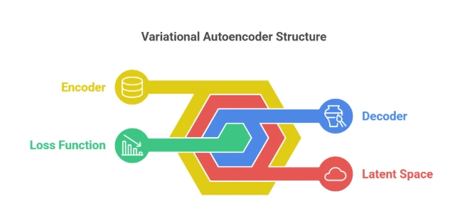
The VAE consists of two main components:
- Encoder: This neural network maps input data to a distribution in the latent space, typically producing the mean and variance of a Gaussian distribution.
- Decoder: This network takes samples from the latent space and reconstructs the original data from these samples.
The VAE is trained by maximizing a variational lower bound on the data likelihood, which combines:
- Reconstruction loss: Measures how well the decoder reconstructs the input data.
- KL divergence: Regularizes the latent space, ensuring that the learned distribution is close to a prior distribution (usually Gaussian).
The VAE enables the generation of new, realistic data by sampling from the learned latent space, making it highly useful for tasks such as image generation, anomaly detection, and data synthesis.
The Architecture of Variational Autoencoder
The Encoder, the Latent Space, and the Decoder are the three main parts that make up the design of a Variational Autoencoder (VAE). Each part is very important for learning how the data is likely to be represented and making new samples that are similar.
1. Encoder
- Purpose: The encoder takes the source data xx, which could be a picture or a list of items, and maps it to a probabilistic distribution in the hidden space.
- Structure: Usually, the encoder is made up of several layers of neural networks, such as fully linked layers or convolutional layers for images. Two vectors make up the end output:
- Mean vector (μmu): Represents the central tendency of the latent variables.
- Log variance vector (log(σ2)log(sigma^2)): Represents the uncertainty or spread of the latent distribution.
- Mathematical Mapping: The encoder produces a distribution q(z∣x)q(z|x) from which the latent variables zz are sampled.
2. Latent Space
- Purpose: The latent space is a continuous, low-dimensional space that captures the underlying structure of the data. The encoder doesn’t produce a single point in this space, but rather a distribution, usually a Gaussian.
- Sampling: A key concept in VAEs is reparameterization. Instead of sampling directly from q(z∣x)q(z|x), the model samples from a standard Gaussian and then applies the mean and variance to produce zz. This allows gradients to flow through the sampling process during backpropagation. The reparameterization trick is: z=μ(x)+σ(x)⋅ϵz = mu(x) + sigma(x) cdot epsilon where ϵ∼N(0,I)epsilon sim N(0, I) is a random variable sampled from the standard Gaussian.
3. Decoder
- Purpose: The decoder maps the latent variables zz back to the original data space. The decoder reconstructs the input data from the sampled latent code.
- Structure: Like the encoder, the decoder is typically a neural network composed of fully connected or convolutional layers. The decoder reconstructs the data x^hat{x}, which is an approximation of the original input xx.
- Mathematical Mapping: The decoder learns the distribution p(x∣z)p(x|z), which describes the probability of observing xx given the latent code zz.
Loss Function
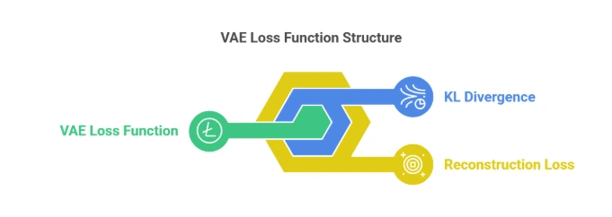
The VAE is trained using a loss function that consists of two terms:
- Reconstruction Loss: Measures how well the decoder reconstructs the input data. This is typically the mean squared error (MSE) or binary cross-entropy loss. Lrecon=Eq(z∣x)[logp(x∣z)]mathcal{L}_{text{recon}} = mathbb{E}_{q(z|x)}[log p(x|z)]
- KL Divergence Loss: Regularizes the latent space by ensuring that the learned distribution q(z∣x)q(z|x) is close to a prior distribution, often a standard Gaussian p(z)p(z). This term penalizes deviations from the prior. LKL=DKL(q(z∣x)∥p(z))mathcal{L}_{text{KL}} = D_{text{KL}}(q(z|x) parallel p(z))
The total VAE Loss is the sum of the reconstruction loss and the KL divergence:
LVAE=Lrecon+LKLmathcal{L}_{text{VAE}} = mathcal{L}_{text{recon}} + mathcal{L}_{text{KL}}
Summary of VAE Architecture:

- Encoder: Maps input data to a probabilistic latent space, producing mean and variance vectors.
- Latent Space: A continuous distribution from which latent variables are sampled.
- Decoder: Reconstructs the original data from the sampled latent variables.
- Loss Function: Combines reconstruction error and KL divergence to train the model.
The VAE can learn a structured, continuous latent space with this architecture. This is helpful for creating new data, finding anomalies, and other jobs that need creating data.
Intuitions About the Regularization
Regularization in VAEs makes sure that the latent space is represented in a meaningful way, which helps the learned model be smooth and general. It’s possible to divide perception into three main parts:
- The loss function in a VAE comprises two components:
- Reconstruction Loss: Encourages the model to accurately reconstruct input data.
- KL Divergence (Regularization): Ensures the learned latent space distribution is close to a prior (usually a standard Gaussian).
- The loss function in a VAE comprises two components:


This balance keeps the model from just remembering the data and encourages a structured latent space that can hold important differences.
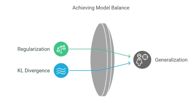
- Preventing Overfitting:
- If you don’t regularize the data, the model might learn too much from the training data and not be able to apply what it has learned to new data.
- The KL divergence regularization keeps things from fitting too well by encouraging smooth changes between hidden representations.
- Ensuring a Continuous and Interpolatable Latent Space:
- Regularization pushes the latent space to follow a known probability distribution (e.g., Gaussian). This makes the latent space more continuous, enabling smooth interpolations and meaningful sampling.
Practical Considerations:
Regularization ensures that:
- The latent variables encode generalizable and disentangled features.
- The generated samples remain coherent and diverse.
- Sampling from the latent space produces realistic data as the space aligns with the prior distribution.
To sum up, regularization helps find a balance between learning from the data and sticking to a probabilistic structure. This is important for making sure that generative modeling in VAEs is stable and easy to understand.
Mathematical Details of VAEs
Variational Autoencoders (VAEs) are probabilistic generative models that learn a hidden representation and then use it to make new data points that are similar to the training data. The mathematical framework is broken down below:
1. Objective of VAEs
The goal of a VAE is to maximize the likelihood p(x)p(x) of the data xx, which is achieved by optimizing the evidence lower bound (ELBO). This involves latent variables zz:
p(x)=∫p(x,z) dzp(x) = int p(x, z) , dz
Since this integral is intractable, VAEs optimize the ELBO:
LELBO=Eq(z∣x)[log⁡p(x∣z)]−KL(q(z∣x)∥p(z))mathcal{L}_{text{ELBO}} = mathbb{E}_{q(z|x)}[log p(x|z)] – text{KL}(q(z|x) | p(z))
2. Components of the ELBO
- Reconstruction Loss (Eq(z∣x)[logp(x∣z)]mathbb{E}_{q(z|x)}[log p(x|z)]):
- Measures how well the decoder reconstructs xx from the latent code zz. It is often modeled as: p(x∣z)∼N(x;μdecoder,σ2I)p(x|z) sim mathcal{N}(x; mu_{text{decoder}}, sigma^2 I) where μdecodermu_{text{decoder}} and σ2sigma^2 are outputs of the decoder.
- KL Divergence (KL(q(z∣x)∥p(z))text{KL}(q(z|x) | p(z))):
- Aligns the posterior q(z∣x)q(z|x) with a prior p(z)p(z), typically a standard Gaussian: KL(q(z∣x)∥p(z))=∫q(z∣x)logq(z∣x)p(z) dztext{KL}(q(z|x) | p(z)) = int q(z|x) log frac{q(z|x)}{p(z)} , dz
3. Latent Variable Approximation (Variational Inference)
Since p(z∣x)p(z|x) is intractable, VAEs approximate it using a parametric distribution q(z∣x)q(z|x), often modeled as:
q(z∣x)∼N(μencoder,σencoder2I)q(z|x) sim mathcal{N}(mu_{text{encoder}}, sigma_{text{encoder}}^2 I)
The encoder network outputs μencodermu_{text{encoder}} and σencodersigma_{text{encoder}}, representing the mean and variance of this Gaussian distribution.
4. Reparameterization Trick
To backpropagate through q(z∣x)q(z|x), the reparameterization trick is used:
z=μencoder+σencoder⊙ϵ,ϵ∼N(0,I)z = mu_{text{encoder}} + sigma_{text{encoder}} odot epsilon, quad epsilon sim mathcal{N}(0, I)
This changes the random picking into a deterministic process, which lets it be differentiable.
5. Training Objective
The ELBO is minimized as:
LVAE=Reconstruction Loss+KL Divergencemathcal{L}_{text{VAE}} = text{Reconstruction Loss} + text{KL Divergence}
In practice:
LVAE=−Eq(z∣x)[logp(x∣z)]+β⋅KL(q(z∣x)∥p(z))mathcal{L}_{text{VAE}} = -mathbb{E}_{q(z|x)}[log p(x|z)] + beta cdot text{KL}(q(z|x) | p(z))
where βbeta is a hyperparameter controlling the trade-off between reconstruction and regularization.
6. Decoder (Generative Model)
The decoder maps latent variables zz back to the data space xx:
p(x∣z)∼N(μdecoder,σ2I)p(x|z) sim mathcal{N}(mu_{text{decoder}}, sigma^2 I)
This is modeled using a neural network.
7. Encoder (Inference Model)
The encoder maps data xx to the latent space zz by producing parameters μencodermu_{text{encoder}} and σencodersigma_{text{encoder}}:
q(z∣x)∼N(μencoder,σencoder2I)q(z|x) sim mathcal{N}(mu_{text{encoder}}, sigma_{text{encoder}}^2 I)
This mathematical framework makes it possible for VAEs to find a good mix between reconstruction quality and a well-structured latent space. This lets data be generated and interpolated in a meaningful way.
Neural Networks in the Model
Neural networks are used a lot in variational autoencoders (VAEs) to describe the encoder and decoder parts. The jobs of these neural networks are to put data into a latent space (encoding) and get data back from the latent space (decoding). Here is a list of their functions and roles:
1. Encoder Network
- Purpose: Encodes the input data xx into a latent representation zz by learning the parameters μencodermu_{text{encoder}} and σencodersigma_{text{encoder}} of the approximate posterior distribution q(z∣x)q(z|x).
- Architecture:
- Input: Raw data xx (e.g., image pixels or text embeddings).
- Hidden Layers: Fully connected (dense), convolutional, or recurrent layers depending on the data type.
- Output:
- μencodermu_{text{encoder}}: Mean of the latent Gaussian distribution.
- σencodersigma_{text{encoder}}: Standard deviation (or log variance) of the latent Gaussian distribution.
- Example:
class Encoder(nn.Module):
    def __init__(self, input_dim, latent_dim):
        super(Encoder, self).__init__()
        self.fc1 = nn.Linear(input_dim, 128)
        self.fc_mu = nn.Linear(128, latent_dim)
        self.fc_logvar = nn.Linear(128, latent_dim)

    def forward(self, x):
        h = F.relu(self.fc1(x))
        mu = self.fc_mu(h)
        logvar = self.fc_logvar(h)
        return mu, logvar
2. Latent Space
- The latent space zz is sampled from a Gaussian distribution defined by μencodermu_{text{encoder}} and σencodersigma_{text{encoder}}: z=μencoder+σencoder⊙ϵ,ϵ∼N(0,I)z = mu_{text{encoder}} + sigma_{text{encoder}} odot epsilon, quad epsilon sim mathcal{N}(0, I)
- The reparameterization trick ensures differentiability during backpropagation.
3. Decoder Network
- Purpose: Decodes the latent variable zz back into the original data space xx to reconstruct the input.
- Architecture:
- Input: Latent variable zz.
- Hidden Layers: Fully connected (dense), transposed convolutional, or recurrent layers.
- Output: Parameters of the reconstruction distribution p(x∣z)p(x|z), often modeled as: p(x∣z)∼N(μdecoder,σ2I)p(x|z) sim mathcal{N}(mu_{text{decoder}}, sigma^2 I)
- For images: Pixel intensities.
- For text: Token probabilities.
- Example:
class Decoder(nn.Module):
    def __init__(self, latent_dim, output_dim):
        super(Decoder, self).__init__()
        self.fc1 = nn.Linear(latent_dim, 128)
        self.fc_out = nn.Linear(128, output_dim)

    def forward(self, z):
        h = F.relu(self.fc1(z))
        x_reconstructed = torch.sigmoid(self.fc_out(h))
        return x_reconstructed
4. Loss Functions
- Reconstruction Loss: Measures the difference between the input xx and reconstructed output x^hat{x}. For images: Lreconstruction=−Eq(z∣x)[logp(x∣z)]mathcal{L}_{text{reconstruction}} = -mathbb{E}_{q(z|x)}[log p(x|z)]
- Typically a Mean Squared Error (MSE) or Binary Cross-Entropy (BCE) loss.
- KL Divergence: Regularizes the latent space by aligning q(z∣x)q(z|x) with the prior p(z)p(z): LKL=KL(q(z∣x)∥p(z))mathcal{L}_{text{KL}} = text{KL}(q(z|x) | p(z))
5. Combined Model
- Both the encoder and the decoder are put together in a single model that is adjusted together.
- Example:
class VAE(nn.Module):
    def __init__(self, input_dim, latent_dim):
        super(VAE, self).__init__()
        self.encoder = Encoder(input_dim, latent_dim)
        self.decoder = Decoder(latent_dim, input_dim)

    def forward(self, x):
        mu, logvar = self.encoder(x)
        std = torch.exp(0.5 * logvar)
        z = mu + std * torch.randn_like(std)  # Reparameterization
        x_reconstructed = self.decoder(z)
        return x_reconstructed, mu, logvar
6. Training the VAE
To train the VAE, the total loss is kept as low as possible:
LVAE=Lreconstruction+LKLmathcal{L}_{text{VAE}} = mathcal{L}_{text{reconstruction}} + mathcal{L}_{text{KL}}
- Example Training Loop:
optimizer = torch.optim.Adam(vae.parameters(), lr=1e-3)
for epoch in range(num_epochs):
    for x in dataloader:
        x_reconstructed, mu, logvar = vae(x)
        reconstruction_loss = F.binary_cross_entropy(x_reconstructed, x, reduction='sum')
        kl_loss = -0.5 * torch.sum(1 + logvar - mu.pow(2) - logvar.exp())
        loss = reconstruction_loss + kl_loss
        optimizer.zero_grad()
        loss.backward()
        optimizer.step()
Variational Autoencoder Execution
There are several steps needed to run a Variational Autoencoder (VAE), such as defining the design, training the model, and evaluating it. Here is an organized outline of how to carry out a VAE:
1. Setup
Install the necessary libraries:
pip install torch torchvision matplotlib
Import required packages:
import torch
import torch.nn as nn
import torch.optim as optim
from torch.utils.data import DataLoader
from torchvision import datasets, transforms
import matplotlib.pyplot as plt
2. Define the VAE Components
Encoder
The encoder maps the input data xx to the latent space zz:
class Encoder(nn.Module):
    def __init__(self, input_dim, latent_dim):
        super(Encoder, self).__init__()
        self.fc1 = nn.Linear(input_dim, 128)
        self.fc_mu = nn.Linear(128, latent_dim)
        self.fc_logvar = nn.Linear(128, latent_dim)

    def forward(self, x):
        h = torch.relu(self.fc1(x))
        mu = self.fc_mu(h)
        logvar = self.fc_logvar(h)
        return mu, logvar
Decoder
The decoder reconstructs xx from the latent variable zz:
class Decoder(nn.Module):
    def __init__(self, latent_dim, output_dim):
        super(Decoder, self).__init__()
        self.fc1 = nn.Linear(latent_dim, 128)
        self.fc_out = nn.Linear(128, output_dim)

    def forward(self, z):
        h = torch.relu(self.fc1(z))
        x_reconstructed = torch.sigmoid(self.fc_out(h))
        return x_reconstructed
VAE
Combine the encoder and decoder:
class VAE(nn.Module):
    def __init__(self, input_dim, latent_dim):
        super(VAE, self).__init__()
        self.encoder = Encoder(input_dim, latent_dim)
        self.decoder = Decoder(latent_dim, input_dim)

    def forward(self, x):
        mu, logvar = self.encoder(x)
        std = torch.exp(0.5 * logvar)
        z = mu + std * torch.randn_like(std)  # Reparameterization trick
        x_reconstructed = self.decoder(z)
        return x_reconstructed, mu, logvar
3. Loss Function
The VAE loss includes both reconstruction loss and KL divergence:
def vae_loss(x, x_reconstructed, mu, logvar):
    reconstruction_loss = nn.functional.binary_cross_entropy(x_reconstructed, x, reduction='sum')
    kl_loss = -0.5 * torch.sum(1 + logvar - mu.pow(2) - logvar.exp())
    return reconstruction_loss + kl_loss
4. Data Preparation
Use a dataset such as MNIST:
transform = transforms.Compose([transforms.ToTensor(), transforms.Lambda(lambda x: x.view(-1))])
mnist = datasets.MNIST(root='./data', train=True, download=True, transform=transform)
dataloader = DataLoader(mnist, batch_size=64, shuffle=True)
5. Training the VAE
input_dim = 28 * 28  # For MNIST
latent_dim = 10
vae = VAE(input_dim, latent_dim)
optimizer = optim.Adam(vae.parameters(), lr=1e-3)

for epoch in range(10):
    total_loss = 0
    for x, _ in dataloader:
        x_reconstructed, mu, logvar = vae(x)
        loss = vae_loss(x, x_reconstructed, mu, logvar)
        optimizer.zero_grad()
        loss.backward()
        optimizer.step()
        total_loss += loss.item()
    print(f"Epoch {epoch + 1}, Loss: {total_loss / len(dataloader.dataset):.4f}")
6. Visualizing the Results
Reconstructed Images
vae.eval()
with torch.no_grad():
    for x, _ in dataloader:
        x_reconstructed, _, _ = vae(x)
        break

x = x.view(-1, 28, 28)
x_reconstructed = x_reconstructed.view(-1, 28, 28)

fig, axes = plt.subplots(1, 2, figsize=(10, 5))
axes[0].imshow(x[0].cpu(), cmap='gray')
axes[0].set_title("Original Image")
axes[1].imshow(x_reconstructed[0].cpu(), cmap='gray')
axes[1].set_title("Reconstructed Image")
plt.show()
7. Latent Space Visualization
Visualize the latent space for 2D latent variables:
latent_dim = 2
vae = VAE(input_dim, latent_dim)

# Train the VAE first

with torch.no_grad():
    z = []
    labels = []
    for x, y in dataloader:
        mu, _ = vae.encoder(x)
        z.append(mu)
        labels.append(y)
    z = torch.cat(z).cpu().numpy()
    labels = torch.cat(labels).cpu().numpy()

plt.scatter(z[:, 0], z[:, 1], c=labels, cmap='tab10', s=5)
plt.colorbar()
plt.title("Latent Space Visualization")
plt.show()
This process shows how to run a VAE from the description stage to the visualization stage.
Visualization of Latent Space
Visualizing the latent space of a Variational Autoencoder (VAE) provides insights into how the model organizes data in its compressed representation. Here’s a step-by-step guide to perform latent space visualization:
1. Preliminary Setup
You need a trained VAE with a 2D latent space (for easy visualization).
2. Generate Latent Space Embeddings
Use the encoder to extract latent space embeddings for a dataset.
import matplotlib.pyplot as plt
import torch

# Function to extract latent space embeddings
def extract_latent_space(vae, dataloader):
    vae.eval()
    z = []
    labels = []
    with torch.no_grad():
        for x, y in dataloader:
            mu, _ = vae.encoder(x)
            z.append(mu)
            labels.append(y)
    z = torch.cat(z).cpu().numpy()
    labels = torch.cat(labels).cpu().numpy()
    return z, labels
3. Visualize Latent Space
Plot the 2D latent space using a scatter plot.
# Extract latent embeddings
z, labels = extract_latent_space(vae, dataloader)

# Plot the latent space
plt.figure(figsize=(8, 6))
scatter = plt.scatter(z[:, 0], z[:, 1], c=labels, cmap='tab10', s=10)
plt.colorbar(scatter, label="Class Label")
plt.title("Latent Space Visualization")
plt.xlabel("Latent Dimension 1")
plt.ylabel("Latent Dimension 2")
plt.grid()
plt.show()
4. Generate Data from Latent Space
Grid-sample the latent space and decode for visualization.
import numpy as np

# Generate grid points
grid_x = np.linspace(-3, 3, 20)
grid_y = np.linspace(-3, 3, 20)
grid = torch.tensor([[x, y] for x in grid_x for y in grid_y], dtype=torch.float)

# Decode grid points to images
vae.eval()
with torch.no_grad():
    generated = vae.decoder(grid).view(-1, 28, 28).cpu()

# Visualize reconstructed grid
fig, axes = plt.subplots(len(grid_x), len(grid_y), figsize=(10, 10))
for i, ax_row in enumerate(axes):
    for j, ax in enumerate(ax_row):
        ax.imshow(generated[i * len(grid_y) + j], cmap="gray")
        ax.axis("off")
plt.tight_layout()
plt.show()
This way of looking at latent spaces blends being able to interpret and being creative.
Types of Variational Autoencoder
Variational Autoencoders (VAEs) are powerful generative models that learn to represent input data in a probabilistic latent space and generate new, similar samples from it. While the basic VAE architecture is foundational, multiple types and variants of VAEs have emerged to handle different tasks, improve generative quality, or model more complex distributions.
Let’s explore the key types of VAEs and how they differ.
1. Vanilla VAE
This is the original and most common form of a VAE.
- Encoder maps input data to a mean and variance of a Gaussian distribution.
- Decoder reconstructs data from sampled latent vectors.
- Uses the KL divergence to regularize the latent space.
Use cases: Image generation, anomaly detection, data compression.
Limitations: Generated outputs may be blurry; assumes a simple Gaussian latent space.
2. Conditional VAE (CVAE)
A Conditional VAE learns to generate data conditioned on some auxiliary information such as labels or categories.
- Both encoder and decoder receive the conditioning variable.
- Useful for controlled generation (e.g., generating a digit ‘3’ from MNIST).
Example:
# During training
encoder_input = tf.concat([x, y], axis=1)
decoder_input = tf.concat([z_sample, y], axis=1)
Use cases: Style transfer, text-to-image generation, guided synthesis.
3. β-VAE (Beta-VAE)
Introduces a β hyperparameter to control the trade-off between reconstruction accuracy and latent space disentanglement.
- Loss becomes: Reconstruction Loss + β * KL Divergence
- Higher β encourages disentanglement but may reduce reconstruction quality.
Key benefit: Encourages disentangled representations—different latent variables learn to represent different factors (e.g., object shape, size, orientation).
Use cases: Interpretable generative models, unsupervised feature learning.
4. Vector Quantized VAE (VQ-VAE)
VQ-VAEs use discrete latent variables instead of continuous ones.
- Instead of sampling from a Gaussian, the encoder output is matched to a nearest codebook vector.
- Combines the strengths of VAEs with the discrete nature of models like autoregressive transformers.
Advantages:
- Better suited for discrete data (e.g., text, audio tokens).
- Used in powerful generative models like VQGAN, DALLE-2, and Jukebox.
5. Hierarchical VAE (HVAE)
Uses multiple layers of latent variables to model complex data distributions.
- Each layer captures features at different abstraction levels.
- Allows modeling of more expressive and high-dimensional data.
Use cases: Complex image and video generation, hierarchical text modeling.
6. Discrete VAE / Categorical VAE
Instead of using a Gaussian distribution in the latent space, these models use categorical or discrete latent variables.
- Often optimized using techniques like Gumbel-Softmax.
- Can handle non-continuous structure in data.
Use cases: Clustering, symbolic reasoning, structured data generation.
7. Semi-supervised VAE
These VAEs handle both labeled and unlabeled data during training.
- Extend the VAE framework to include class labels as part of the latent space.
- Can perform classification and generation simultaneously.
Use cases: Scenarios with limited labeled data, such as medical imaging or text classification.
8. Denoising VAE
Trains the model to reconstruct clean data from noisy inputs, increasing robustness.
- Inspired by denoising autoencoders.
- Helps the model learn better latent representations that are robust to input noise.
Use cases: Image denoising, noise-robust generation.
Variational Autoencoder vs Traditional Autoencoder
Autoencoders are neural networks that learn to compress data into a lower-dimensional representation (encoding) and then reconstruct it back to its original form (decoding). However, not all autoencoders are the same. The Traditional Autoencoder and the Variational Autoencoder (VAE) differ fundamentally in their architecture, purpose, and capabilities.
1. Purpose
| Feature | Traditional Autoencoder | Variational Autoencoder (VAE) |
| Main Goal | Dimensionality reduction or reconstruction | Generative modeling and data generation |
| Output Type | Best reconstruction of input | New data samples from learned distribution |
2. Latent Space Representation
- Traditional Autoencoder learns deterministic latent vectors.
- VAE learns a probabilistic distribution over the latent space (usually Gaussian), allowing for sampling and interpolation.
Traditional: Input → Encoded Vector → Output
VAE: Input → μ, σ → Sample z ~ N(μ, σ) → Output
This stochastic sampling in VAE allows it to generate diverse outputs even for similar inputs.
3. Mathematical Foundation
- Traditional Autoencoders minimize only the reconstruction loss (e.g., Mean Squared Error).
- VAEs minimize a combined loss:
Total Loss = Reconstruction Loss + KL Divergence
The KL Divergence ensures the latent space follows a known distribution, typically a standard normal distribution, enabling smooth interpolation and sampling.
4. Generative Capability
- Traditional Autoencoders are not inherently generative—you cannot easily sample meaningful new data from the latent space.
- VAEs are designed for generation—you can sample a vector from the latent space and decode it into realistic data.
5. Architecture Differences
| Component | Traditional Autoencoder | VAE |
| Encoder Output | Latent vector | Mean and variance of distribution |
| Decoder Input | Latent vector | Sampled vector from the distribution |
| Sampling Step | Not applicable | Uses reparameterization trick |
6. Code Example: Key Difference
Here’s a simplified PyTorch-style snippet showing the difference in encoder output:
Traditional Autoencoder:
latent = encoder(x) # Direct encoding
output = decoder(latent)
Variational Autoencoder:
mu, logvar = encoder(x) # Learn distribution parameters
std = torch.exp(0.5 * logvar)
z = mu + std * torch.randn_like(std) # Reparameterization trick
output = decoder(z)
How VAEs could be used in the Future
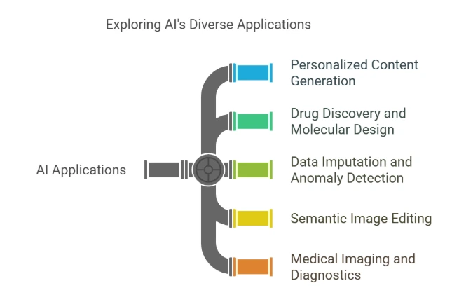
- By learning from user data, VAEs can make images, songs, or media that are specific to each person’s tastes.
- Drug Discovery and Molecular Design
- VAEs can look into molecular latent spaces to create new drugs with specific qualities, which would completely change the pharmaceutical industry.
- Data Imputation and Anomaly Detection
- VAEs can find problems in healthcare, banking, or IoT systems and fill in missing data.
- Semantic Image Editing
- VAEs let you finetune picture editing, like changing the style or features, which makes them useful for making content.
- Medical Imaging and Diagnostics
- VAEs make medical pictures better by removing noise, reconstructing images, or making fake images that can help with diagnosis.

Conclusion
VAEs, which combine deep learning with statistical frameworks to model complex data distributions quickly and accurately, have become a powerful tool in generative modeling. They can work in a wide range of industries because they can produce high-quality outputs, learn useful latent representations, and adapt to different tasks. VAEs have a huge amount of potential for innovation, from making personalized content to medical diagnosis and drug finding. As study grows, combining VAEs with other cutting-edge technologies could open up new options. This would help AI applications move forward and make the future more creative, efficient, and smart. See how CycleGAN enables stunning image-to-image translation without paired datasets.
Generative AI enables machines to generate realistic content by analyzing data. A Gen AI certification equips learners with expertise in deep learning, neural networks, and AI-driven innovation, opening doors to advanced career opportunities in artificial intelligence.
Frequently Asked Questions
1. What is the structure of a variational autoencoder?
VAE stands for Variational Autoencoder. It is a generative model with two main parts: an encoder and a decoder. Using probability, the encoder maps the input data into a hidden variable space (distribution). The decoder then uses the latent factors to put together the input data again. VAEs are different from regular autoencoders because they assume that the data comes from a distribution, usually a Gaussian one. This gives the hidden space a probabilistic structure.
2. What is the architecture of the variational autoencoder decoder?
Usually, a neural network is the decoder in a VAE. It gets the latent variables (sampled from the latent space) and puts together the original input data. The decoder’s design is the same as the encoder’s, but it works backward. It usually has layers, such as fully connected layers or convolutional layers for image data. It connects the hidden variable to the original data space using activation functions such as ReLU, Sigmoid, or Tanh, depending on the type of output (for example, continuous or binary data).
3. What is a variational autoencoder?
A Variational Autoencoder (VAE) is a type of deep learning model that learns to make new data by modeling the chance distribution of the data it is given. The standard autoencoder is built on top of this one, but this one learns to show the data as a distribution instead of a fixed code. The VAE uses a probabilistic method to make sure that the latent space is continuous and set up in a way that makes it possible to create new data points that are similar.
4. What are the components of a variational autoencoder?
Several important parts make up a Variational Autoencoder (VAE):
An encoder is a type of neural network that takes in data, maps it into a latent variable space, and then gives back the distribution’s mean and range.
- Latent Variables: These are the data’s probabilistic representations, which are usually described as a Gaussian distribution.
- Decoder: A neural network that puts together the data from the latent variables that were collected.
- Loss Function: It has two parts: a reconstruction loss that checks how well the data was reconstructed and a regularization loss (KL divergence) that makes sure the latent space follows a prior distribution, which is usually Gaussian.