R Programming – Beginners Guide To R Programming Language

R Programming For Beginners | R Programming Language Tutorial | Edureka

So let’s move forward and look at the first concept of R Programming – Variables.

R Programming: Variables

Variables are nothing but a name to a memory location containing a value.  A variable in R can store Numeric values, Complex Values, Words, Matrices and even a Table. Surprising, right?

The above image shows us how variables are created and how they are stored in different memory blocks. In R, we don’t have to declare a variable before we use it, unlike other programming languages like Java, C, C++, etc.

Let us move forward and try to understand what is a Data type and the various Data types supported in R.

R Programming: Data Types 

In R, a variable itself is not declared of any data type, rather it gets the data type of the R object assigned to it. So R is called a dynamically typed language, which means that we can change a data type of the same variable again and again when using it in a program.

Data Types specifies which type of value a variable has and what type of mathematical, relational or logical operations can be applied to it without causing an error. There are many data types in R, However below are the most frequently used ones:

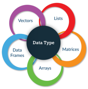Let us now discuss each of these data types individually, starting from Vectors.

Vectors

Vectors are the most basic R data objects and there are six types of atomic vectors. Below are the six atomic vectors:

Logical: It is used to store logical value like TRUE or FALSE.

Numeric: It is used to store both positive and negative numbers including real number.

Eg: 25, 7.1145 , 96547

Integer: It holds all the integer values i.e. all the positive and negative whole numbers.

Eg: 45.479, -856.479 , 0

Complex: These are of the form x + yi, where x and y are numeric and i represents the square root of -1.

Eg: 4+3i

Character: It is used to store either a single character, group of characters(words) or a group of words together. The characters may be defined in either single quotes or double quotes.

Eg: "Edureka", 'R is Fun to learn'.

In general, a vector is defined and initialized in the following manner:

Vtr = c(2, 5, 11 , 24) 

Or

Vtr <- c(2, 5, 11 , 24)

Let us move forward and understand other data types in R.

List

Lists are quite similar to vectors, but Lists are the R objects which can contain elements of different types like − numbers, strings, vectors and another list inside it.

Eg: 

Vtr <- c("Hello", 'Hi','How are you doing')
mylist <- list(Vtr, 22.5, 14965, TRUE) 
mylist

Output:

[[1]]
[1] 'Hello"  "Hi"  "How are you doing"
[[2]]
[1] 22.5
[[3]]
[1] 14965
[[4]]
[1] TRUE

Matrix

Matrix is the R object in which the elements are arranged in a two-dimensional rectangular layout.

The basic syntax for creating a matrix in R is −

matrix(data, nrow, ncol, byrow, dimnames)

Where:

• data is the input vector which becomes the data elements of the matrix.
• nrow is the number of rows to be created.
• ncol is the number of columns to be created.
• byrow is a logical clue. If TRUE, then the input vector elements are arranged by row.
• dimname is the names assigned to the rows and columns.

Example: 

Mymatrix <- matrix(c(1:25), nrow = 5,  ncol = 5, byrow = TRUE) 
Mymatrix

Output:

        [,1]   [,2]   [,3]   [,4]   [,5] 
[1,]    1       2       3     4      5
[2,]    6       7       8     9      10
[3,]    11     12     13    14    15
[4,]    16     17     18    19    20
[5,]    21     22     23    24    25

ARRAY

Arrays in R are data objects which can be used to store data in more than two dimensions. It takes vectors as input and uses the values in the dim parameter to create an array.

The basic syntax for creating an array in R is −

array(data, dim, dimnames)

Where:

• data is the input vector which becomes the data elements of the array.
• dim is the dimension of the array, where you pass the number of rows, column and the number of matrices to be created by mentioned dimensions.
• dimname is the names assigned to the rows and columns.

Example:

Myarray <- array( c(1:16), dim=(4,4,2))
Myarray

Output:

, , 1

      [,1] [,2] [,3] [,4]
[1,]  1    5     9    13
[2,]  2    6    10   14
[3,]  3    7    11   15
[4,]  4    8    12   16

, , 2


      [,1] [,2] [,3] [,4]
[1,]  1    5     9    13
[2,]  2    6    10   14
[3,]  3    7    11   15
[4,]  4    8    12   16

Data Frame

A Data Frame is a table or a two-dimensional array-like structure in which each column contains values of one variable and each row contains one set of values for each column. Below are some of the characteristics of a Data Frame that needs to be considered every time we work with them:

• The column names should be non-empty.
• Each column should contain the same amount of data items.
• The data stored in a data frame can be of numeric, factor or character type.
• The row names should be unique.

Example:

emp_id = c(100:104)
emp_name = c("John","Henry","Adam","Ron","Gary")
dept = c("Sales","Finance","Marketing","HR","R & D")
emp.data <- data.frame(emp_id, emp_name, dept)
emp.data

Output:

   emp_id    emp_name    dept
1 100         John              Sales
2 101         Henry            Finance
3 102         Adam            Marketing
4 103         Ron               HR
5 104         Gary              R & D

So now that we have understood the basic data types of R, it’s time we deep dive into R by understanding the concepts of Data Operators.

R Programming: Data Operators

There are mainly 4 data operators in R, they are as seen below:

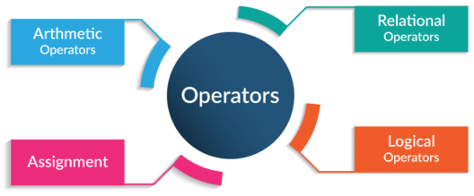
Arithmetic Operators: These operators help us perform the basic arithmetic operations like addition, subtraction, multiplication, etc.

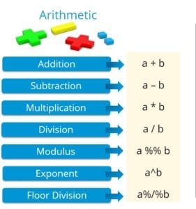
Consider the following example:

num1 = 15
num2 = 20
num3 = 0
#addition
num3 = num1 + num2
num3

#substraction
num3 = num1 - num2
num3

#multiplication
num3= num1 * num2
num3

#division
num3 = num1 / num2
num3

#modulus
num3 = num1 %% num2
num3

#exponent
num1 = 5
num2 = 3
num3 = num1^num2
num3

#floor division
num3 = num1%/%num2
num3

Output:

[1] 35

[1] -5

[1] 300

[1] 0.75

[1] 15

[1] 125

[1] 1

Relational Operators: These operators help us perform the relational operations like checking if a variable is greater than, lesser than or equal to another variable. The output of a relational operation is always a logical value.

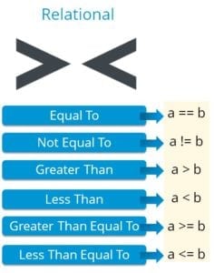
Consider the following examples:

num1 = 15
num2 = 20

#equals to
num3=( num1 == num2 )
num3

#not equal to
num3= ( num1 != num2 )
num3

#lesser than
num3= ( num1 < num2 ) num3 #greater than num3= ( num1 > num2 )
num3

#less than equal to
num1 = 5
num2 = 20
num3 = ( num1 <= num2 ) num3 #greater than equal to num3 = ( num1 >= num2 )
num3

Output:

[1] FALSE

[1] TRUE

[1] TRUE

[1] FALSE

[1] TRUE

[1] FALSE

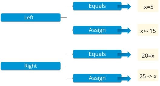
Assignment Operators: These operators are used to assign values to variables in R. The assignment can be performed by using either the assignment operator (<-) or equals operator (=). The value of the variable can be assigned in two ways, left assignment and right assignment.

Logical Operators: These operators compare the two entities and are typically used with boolean (logical) values such as ‘and’, ‘or’ and ‘not’. 

R Programming: Conditional Statements

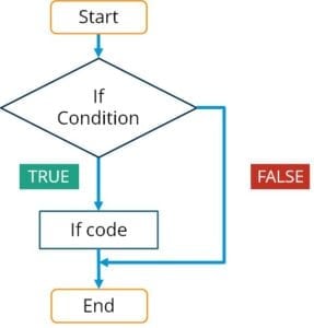1. If Statement: The If statement helps you in evaluating a single expression as part of the flow. To perform this evaluation, you just need to write the If keyword followed by the expression to be evaluated. The below flow diagram will give an idea of how the If statement controls the flow of a code: Consider the following example:
   

num1=10
num2=20

if(num1<=num2){
print("Num1 is less or equal to Num2")

Output:

[1] "Num1 is less or equal to Num2"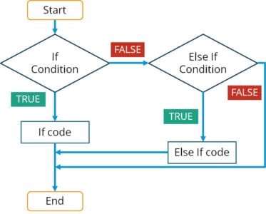

• Else If Statement: The Else if statement helps you in extending branches to the flow created by the If statement and give you the opportunity to evaluate multiple conditions by creating new branches of flow. The below flow will give you an idea of how the else if statement branches the flow of the code:
  
  Consider the following example:

   
  Num1 = 5 
  Num2 = 20
  if (Num1 < Num2) print("Num1 is lesser than Num2") } else if( Num1 > Num2){
    print( "Num2 is lesser than Num1") }
  else if("Num1 == Num2){
          print("Num1 and Num2 are Equal") }
  

  Output:

  [1] "Num1 is lesser than Num2"

   

• Else Statement: The else statement is used when all the other expressions are checked and found invalid. This will be the last statement that gets executed as part of the If – Else if branch. Below flow will give you a better idea on how Else alters the flow of the code:

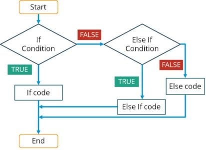
Consider the following example:

 
Num1 = 5 
Num2 = 20
if (Num1< Num2) print("Num1 is lesser than Num2") } else if( Num1 > Num2){
  print( "Num2 is lesser than Num1") }
else
  print("Num1 and Num2 are Equal") }

Output:

[1] "Num1 and Num2 are Equal"

R Programming: Loops

A loop statement allows us to execute a statement or group of statements multiple times. There are mainly 3 types of loops in R:

1. repeat Loop: It repeats a statement or group of statements while a given condition is TRUE. Repeat loop is the best example of an exit controlled loop where the code is first executed and then the condition is checked to determine if the control should be inside the loop or exit from it. Below is the flow of control in a repeat loop:
   Let us look at the example below to understand how we can use repeat loop to add n numbers till the sum reaches exceeds 100:

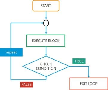
   x=2
   repeat {
   x= x^2
   print(x)
   if(x>100) {
   break
   }
   

   Output:

   [1] 4
   
   [1] 16
   
   [1] 256

2. while Loop: It helps to repeats a statement or group of statements while a given condition is TRUE. While loop, when compared to the repeat loop is slightly different, it is an example of an entry controlled loop where the condition is first checked and only if the condition is found to be true does the control be delivered inside the loop to execute the code. Below is the flow of control in a while loop:
   Let us look at the example below to add the sum of squares for the first 10 numbers and understand how the while loop works better:

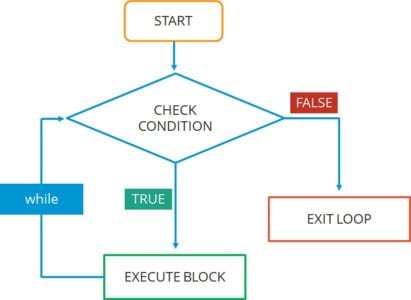
   num = 1
   sumn = 0
   
   while (num<=11){
    sumn =(sumn+ (num^2)
    num = num+1
    print(sumn)
   }
   

   
   Output:

   [1] 1
   [1] 5
   [1] 14
   [1] 30
   [1] 55
   [1] 91
   [1] 140
   [1] 204
   [1] 285
   [1] 385
   [1] 506

3. for Loop: It is used to repeats a statement or group of for a fixed number of times. Unlike repeat and while loop, the for loop is used in situations where we are aware of the number of times the code needs to executed beforehand. It is similar to the while loop where the condition is first checked and then only does the code written inside get executed. Lets see the flow of control of for loop now:

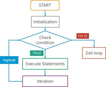
Let us now look at an example where we will be using the for loop to print the first 10 numbers:

 

for(x in 1:10){
print(x)
}

Output:

[1] 1
[1] 2
[1] 3
[1] 4
[1] 5
[1] 6
[1] 7
[1] 8
[1] 9
[1] 10

R Programming: Functions

A function is a block of organized, reusable code that is used to perform a single, related action. There are mainly two types of functions in R:

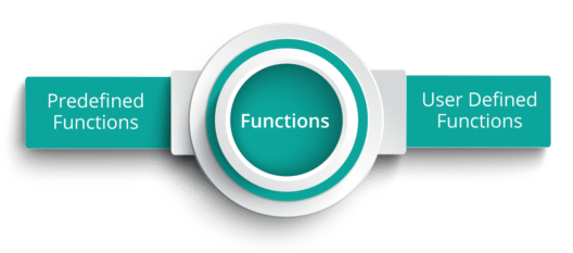Predefined Functions: These are built in functions that can be used by the user to make their work easier. Eg: mean(x), sum(x) ,sqrt(x),toupper(x), etc.

User Defined Functions: These functions are created by the user to meet a specific requirement of the user. The below is the syntax for creating a function in R:

function_name <–function(arg_1, arg_2, …) { 

//Function body 

}

Consider the following example of a simple function for generating the sum of the squares of 2 numbers:

sum_of_square <- function(x,y) {
x^2 + y^2
}
sum_of_sqares(3,4)

Output:
 [1] 25

I hope you have enjoyed reading this R programming blog. We have covered all the basics of R in this tutorial, so you can start practicing now. After this R programming blog, I will be coming up with more blogs on R for Analytics so stay tuned.

Now that you have understood basics of R, check out the R Certification Training by Edureka, a trusted online learning company with a network of more than 250,000 satisfied learners spread across the globe. Edureka’s Data Analytics with R training will help you gain expertise in R Programming, Data Manipulation, Exploratory Data Analysis, Data Visualization, Data Mining, Regression, Sentiment Analysis and using RStudio for real life case studies on Retail, Social Media.

Got a question for us? Please mention it in the comments section of this “R Programming” blog and we will get back to you as soon as possible.