LSTM Explained: Key to Sequential Data in AI

Long Short-Term Memory Networks (LSTM) use artificial neural networks (ANNs) in the domains of deep learning and artificial intelligence (AI). Unlike regular feed-forward neural networks, also known as recurrent neural networks, these networks have feedback connections. Speech recognition, machine translation, robotic control, video games, healthcare, and unsegmented, connected handwriting recognition are some of the uses for Long Short Term Memory networks (LSTM).

What is LSTM?

Deep learning extensively uses the recurrent neural network (RNN) architecture known as LSTM (Long Short-Term Memory). This architecture is perfect for sequence prediction tasks because it is very good at capturing long-term dependencies.

By including feedback connections, LSTM differs from conventional neural networks in that it can process entire data sequences rather than just individual data points. This makes it highly effective in understanding and predicting patterns in sequential data like time series, text, and speech.

Through the discovery of important insights from sequential data, LSTM has developed into a potent tool in deep learning and artificial intelligence that has enabled breakthroughs in various fields. 

You now understand what LSTM is. Next, we’ll examine why it’s important.

Why is LSTM Necessary?

LSTM’s ability to avoid the problem of vanishing gradients and successfully maintain large regions of dependency span in sequential data is undoubtedly a crucial feature that sets it apart from earlier conventional RNNs. For tasks where long-range relationships are essential, such as language modeling, time series analysis, and speech recognition, its specialized memory cells and gating machinery have proven useful. 

Let’s see what RNN is.

What is RNN?

One kind of neural network intended for processing sequential data is a recurrent neural network (RNN). These networks are capable of analyzing temporally oriented data, including text, speech, and time series. They accomplish this by using a hidden state that is passed from one timestep to the next. At every timestep, the input and the previous hidden state are used to update the secret state. RNNs have trouble identifying long-term dependencies in sequential data, but they can locate short-term dependencies. 

Next, we’ll examine what LSTM Architecture is.

LSTM Architecture

In the introduction to long short-term memory, we discovered that it solves the vanishing gradient problem that RNNs encounter. In this section, we will examine how it does so by understanding the LSTM architecture. In general, LSTM functions similarly to an RNN cell. This is the LSTM network’s internal operation. Three components make up the LSTM network architecture, as seen in the image below, and each one serves a distinct purpose. 

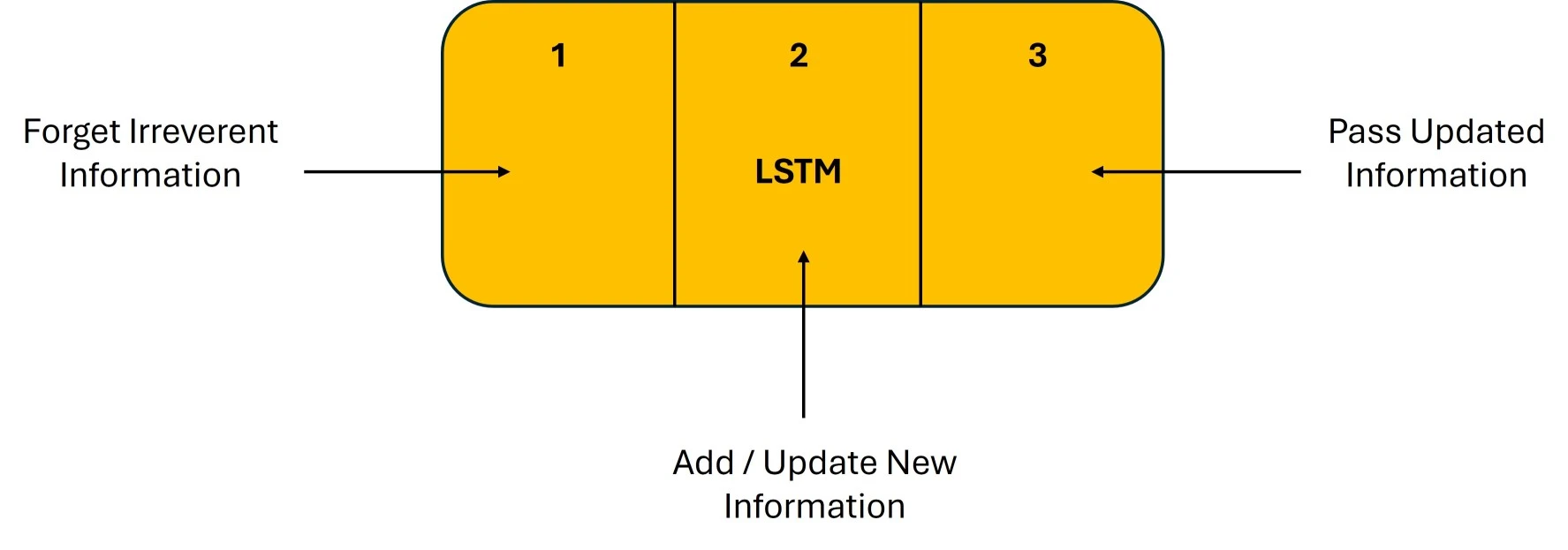The Logic Behind LSTM

The first section determines if the data from the prior timestamp should be retained or if it is unimportant and should be forgotten. The cell attempts to learn new information from the input in the second section. Finally, the cell moves the updated data from the current timestamp to the subsequent timestamp in the third section. This LSTM cycle is regarded as a single-time step. 

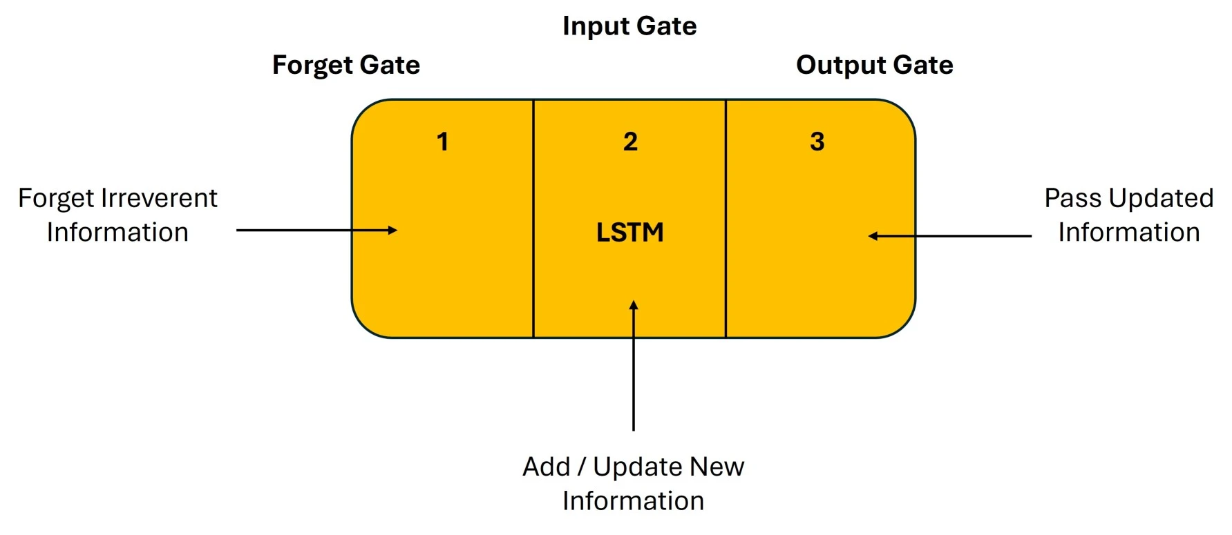
Gates are these three components of an LSTM unit. They regulate the information that enters and exits the memory cell, also known as the LSTM cell. The input gate is the second gate, the output gate is the last, and the forget gate is the first. In a conventional feedforward neural network, an LSTM unit made up of these three gates and a memory cell, also known as an LSTM cell, can be thought of as a layer of neurons, with each neuron having a current state and a hidden layer. 

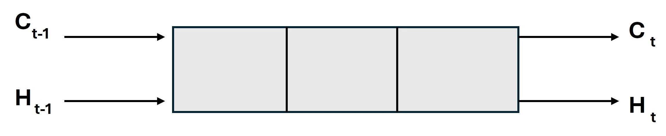
An LSTM, like a basic RNN, has a hidden state, where Ht is the hidden state of the current timestamp and H(t-1) is the hidden state of the previous timestamp. Additionally, C(t-1) and C(t) for the prior and current timestamps, respectively, represent the cell state of LSTM.

In this case, short-term memory refers to the hidden state, while long-term memory refers to the cell state. Take a look at the image below.

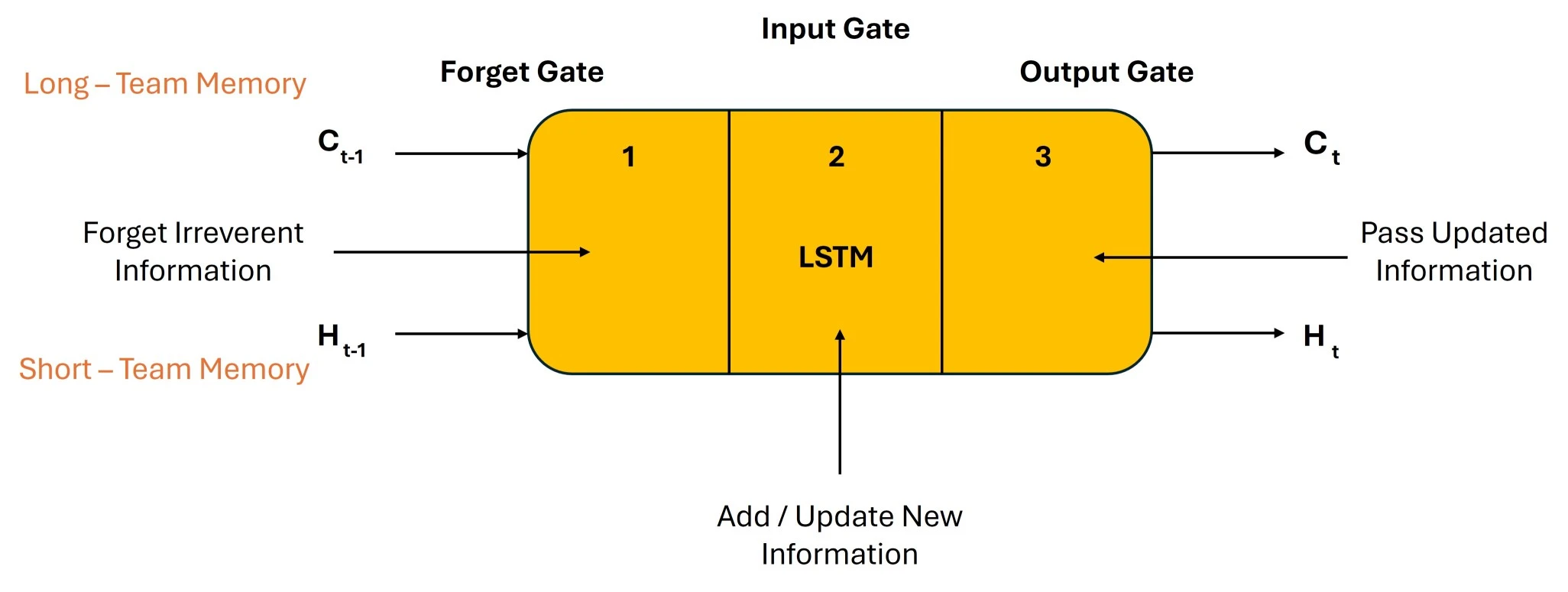It is noteworthy that the cell state carries all of the timestamps and the information.

Let’s examine how LTSM works.

LTSM Working

• Forget Gate
• Input Gate
• Output Gate

The chain structure of the LSTM architecture comprises four neural networks and various memory blocks known as cells.

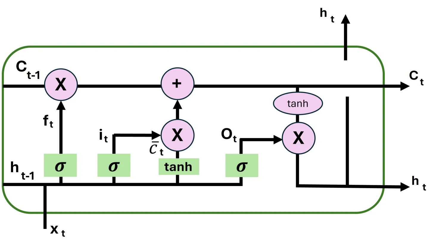The cells store information, and the gates carry out memory manipulation. Three gates are present. 

Forget Gate

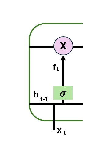
The forget gate eliminates data that is no longer relevant in the cell state. The gate receives two inputs, xt (input at that specific moment) and ht-1 (output from the previous cell), which are multiplied by weight matrices before bias is added. An activation function is applied to the resultant, producing a binary output. A piece of information is lost if the production for a given cell state is 0, but it is kept for later use if the output is 1. The forget gate’s equation is:

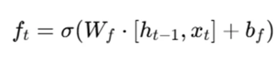
Where W_f denotes the weight matrix connected to the forget gate.

• The concatenation of the current input and the previous hidden state is indicated by [h_t-1, x_t].
• The forget gate’s bias is denoted by b_f.
• The sigmoid activation function is denoted by σ. 

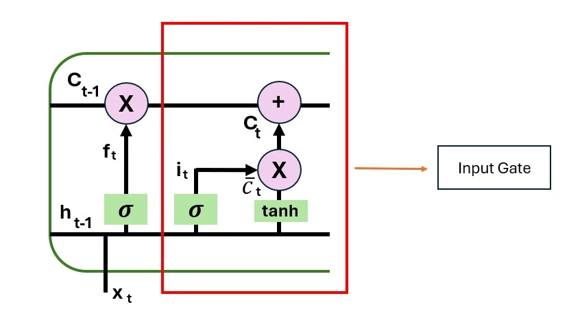
Input gate

The input gate is responsible for adding valuable information to the cell state. Initially, the sigmoid function is used to regulate the data, and the inputs ht-1 and xt are used to filter the values to be remembered in a manner akin to the forget gate. The tanh function is then used to create a vector that contains all of the possible values from ht-1 and xt and has an output ranging from -1 to +1. Finally, the useful information is obtained by multiplying the vector values by the regulated values. The input gate’s equation is

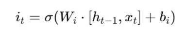
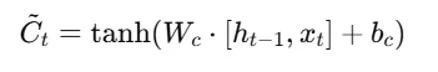
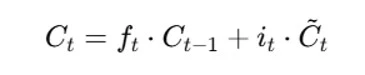
We ignore the information we previously decided to ignore and multiply the previous state by ft. We then incorporate it∗Ct. After accounting for the amount we decided to change for each state value, this shows the revised candidate values.

where

• ⊙ denotes element-wise multiplication
• tanh is the tanh activation function

Output gate

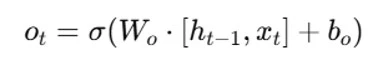
The output gate is responsible for extracting useful information from the current cell state to be presented as output. The tanh function is first applied to the cell to create a vector. The data is then filtered by the values to be remembered using inputs ht-land xt and controlled by the sigmoid function. Finally, to be sent as an output and input to the following cell, the vector and regulated values are multiplied. The output gate’s equation is: 

We will now examine the various applications of LSTM.

Applications of LSTM

Several well-known uses for LSTM include:

• Language Modeling: LSTMs have been applied to tasks involving natural language processing, including text summarization, machine translation, and language modeling. By teaching them the relationships between words in a sentence, they can be trained to produce grammatically sound and coherent sentences.
• Speech Recognition: LSTMs have been applied to speech recognition tasks like spoken command recognition and speech-to-text transcription. They can be trained to identify speech patterns and associate them with the relevant text.
• Time Series Forecasting: LSTMs have been applied to time series forecasting tasks, including energy consumption, weather forecasting, and stock price prediction. They can predict future events by identifying patterns in time series data. 
• Anomaly Detection: LSTMs have been applied to tasks involving anomaly detection, including network intrusion and fraud detection. They can be taught to recognize unusual patterns in data and mark them as possible abnormalities.
• Recommender Systems: LSTMs have been applied to recommendation tasks like book, music, and movie recommendations. They can identify trends in user behavior and use them to provide tailored suggestions.
• Video Analysis: LSTMs have handled tasks like object detection, activity recognition, and action classification. Video data can be combined with other neural network architectures, such as convolutional neural networks (CNNs), to evaluate video data and extract valuable information. 

Let’s examine the differences between RNN and LSTM.

Difference Between RNN and LSTM

The primary distinction between LSTM and RNN is their capacity to process and learn from sequential data. For many sequential data tasks, LSTMs are the recommended option due to their greater sophistication and ability to manage long-term dependencies. Examine the table below for a comparison of LSTM and RNN.

We will now discuss bidirectional LSTMs, as everyone is aware of the differences between RNN and LSTM.

What are Bidirectional LSTMs?

One kind of recurrent neural network (RNN) architecture that can process input data both forward and backward is called a bidirectional LSTM (Long-Short-Term Memory). In a traditional LSTM, where information only moves from the past to the future, predictions are made using the previous context. However, bidirectional LSTMs can capture dependencies in both directions because the network also takes future context into account. 

The bidirectional LSTM consists of two LSTM layers: one processes the input sequence forward, while the other does the opposite. As a result, the network can concurrently access data from previous and upcoming time steps. Bidirectional LSTMs are, therefore, especially helpful for tasks requiring a thorough comprehension of the input sequence, like named entity recognition, machine translation, and sentiment analysis in natural language processing.

Bidirectional LSTMs combine information from both directions to improve the model’s capacity to identify long-term dependencies and produce more precise predictions in complex sequential data. 

We will then discuss the issue of long-term dependencies in RNN.

Problem with Long-Term Dependencies in RNN

Recurrent neural networks (RNNs) keep a hidden state that records data from earlier time steps to process sequential data. They frequently struggle, though, when learning long-term dependencies, where knowledge from far-off time steps is essential for precise forecasting. This issue is referred to as the “exploding gradient” or “vanishing gradient” problem.

A few typical problems are mentioned below:

• Disappearing Gradient

As gradients are multiplied through the chain of recurrent connections during backpropagation through time, they can get incredibly small, making it difficult for the model to learn dependencies that are separated by a large number of time steps.

• The Gradient Exploding

On the other hand, gradients may blow up during backpropagation, which could cause numerical instability and hinder the model’s ability to converge.

Different Variants on Long Short-Term Memory

Numerous modifications and enhancements to the initial LSTM architecture have been suggested over time.

• LSTM Vanilla

Hochreiter and Schmidhuber first proposed this LSTM architecture. To regulate the information flow, it has memory cells with input, forget, and output gates. The main concept is allowing the network to selectively update and forget data from the memory cell.

• Connections Through Peepholes

The gates in the peephole LSTM are permitted to view both the hidden state and the cell state. This gives the gates additional context information by enabling them to consider the cell state when making decisions.

• Gated Recurrent Unit (GRU)

GRU is a simpler and more computationally efficient alternative to LSTM. It merges the cell state and hidden state and combines the input and forgets gates into a single “update” gate. Despite having fewer parameters than LSTMs, GRUs have demonstrated comparable performance in real-world scenarios. 

Conclusion

This blog discussed the fundamentals of a Long-Short-Term Memory Network (LSM) model and its sequential architecture. Understanding its operation facilitates the design of an LSTM model and improves comprehension. Covering this subject is crucial because LSTM models are frequently employed in artificial intelligence for tasks involving natural language processing, such as machine translation and language modeling. 

We’ll now examine the frequently asked questions in LSTM.

FAQs

1. What do we mean by RNN and LSTM?

RNN, or Recurrent Neural Networks, refers to a specific type of neural net designed for sequencing data, where the results of the previous step are used as input for the next.
Long-short-term memory(LSTM) is a special kind of RNN. It addresses the problem of vanishing gradients by using memory cells and gates to store and manage longer-term dependencies in sequences.

2. State any three reasons why LSTM is great.

LSTM best tackles tasks requiring the modeling of long-term dependencies in sequential data, such as speech recognition, language translation, time series forecasting, and even video analysis.

3. What are LSTM and CNN?

LSTM is a sequential data modeling technique based on prediction and a type of recurrent neural network.
CNN is used mainly for image recognition and processing, as it is focused exclusively on spatial data by the detection of patterns in images.
They are usually combined in video analysis, where a CNN performs feature extraction at each frame, and LSTM captures temporal dependencies.

4. Why LSTM?

LSTMs are preferred over other traditional RNNs because they can learn from long sequences without the problem of vanishing gradients.

5. What are the differences between CNN and LSTM time series?

CNNs are used to catch local patterns in sequence data and often feature extraction for time-series data.
LSTMs have a better capacity for modeling long-term dependency and sequential relationships in time-series data.
While CNN is generally used for feature extraction from time-series data, LSTM may be better for forecasting time series utilizing sequential data modeling.

Our blog post on LSTM Explained: Key to Sequential Data in AI comes to an end here. We have looked at the basic ideas behind Long Short Term Memory networks and how important they are for managing sequential data in a variety of AI applications. This summary has demonstrated the enormous potential of LSTMs in artificial intelligence and offered crucial insights into how they are revolutionizing domains such as healthcare, machine translation, and speech recognition.

You are keen to improve your abilities and advance your professional chances in the quickly expanding field of generative artificial intelligence. If so, you ought to think about signing up for Edureka’s Generative AI Course: Masters Program. This Generative AI course covers Python, Data Science, AI, NLP, Prompt Engineering, ChatGPT, and more, with a curriculum designed by experts based on 5000+ global job trends. This extensive program is intended to provide you with up-to-date knowledge and practical experience.

Do you have any questions or need further information? Feel free to leave a comment below, and we’ll respond as soon as possible!