Data Science with Python Certification Course
- 131k Enrolled Learners
- Weekend
- Live Class
Linear Regression is one of the most widely used Machine Learning algorithms, but despite it’s popularity a lot of us aren’t thorough with the working and implementation of this algorithm. In this blog on Linear Regression In R, you’ll understand the math behind Linear Regression and it’s implementation using the R language.
To get in-depth knowledge on Data Science and the various Machine Learning Algorithms, you can enroll for live Data Science Certification Training by Edureka with 24/7 support and lifetime access.
The following topics will be covered in this blog:
Regression analysis is a statistical, predictive modelling technique used to study the relationship between a dependent variable and one or more independent variables. Let’s try to understand regression analysis with an example.
Let’s say that you’ve been given a housing price data set of New York City. This data set contains information such as, size, locality, number of bedrooms in the house, etc. Your task here is to predict the price of the house by studying the data set given to you. How would you approach such a problem?
Well, it’s quite simple. You’re going to model a relationship between the dependent variable and independent variable.

But what are dependent and independent variables?
The data about the house, such as the number of bedrooms, the size of the house and so on, are known as the independent or predictor variables. These predictor variables are used to predict the response variable.
The response variable in our case is the price of the house. Response variables are also known as dependent variables because their values depend on the values of the independent variable.
So, given the relevant data about the house, our task at hand is to predict the price of a new house. Such problems are solved using a statistical method called Regression Analysis.
Regression analysis is widely used in the business domain for sales or market forecasting, risk analysis, operation efficiency, finding new trends and etc.
There are many regression analysis techniques, but the three most widely used regression models are:
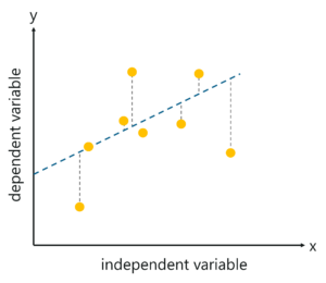
Linear regression is one of the most basic and widely used machine learning algorithms. It is a predictive modelling technique used to predict a continuous dependent variable, given one or more independent variables.
Linear Regression – Linear Regression In R – Edureka
In a linear regression model, the relationship between the dependent and independent variable is always linear thus, when you try to plot their relationship, you’ll observe more of a straight line than a curved one.
The following equation is used to represent a linear regression model:
![]() Linear Regression In R – Edureka
Linear Regression In R – Edureka
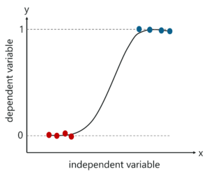
Logistic Regression is a machine learning algorithm used to solve classification problems. It is called ‘Logistic Regression’, because its fundamental technique is quite similar to Linear Regression.
Logistic Regression is a predictive analysis technique used to predict a dependent variable, given a set of independent variables, such that the dependent variable is categorical.
Logistic Regression – Linear Regression In R – Edureka
When I say categorical variable, I mean that, it holds values like 1 or 0, Yes or NO, True or False and so on.
The following equation is used to represent the relationship between the dependent and independent variable in a logistic regression model:

Logistic Regression – Edureka
If you want to learn more about Linear and Logistic Regression, check out this video by our Machine Learning Experts.
This Edureka video on Linear Regression Vs Logistic Regression covers the basic concepts of linear and logistic models.
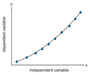
Polynomial Regression is a method used to handle non-linear data. Non-linearly separable data is basically when you cannot draw out a straight line to study the relationship between the dependent and independent variables.
Polynomial Regression – Linear Regression In R – Edureka
Hence in this algorithm, the best fit line is not a straight line, instead, it is a curve that fits into the data points. The reason it is called ‘Polynomial’ regression is that the power of some independent variables is more than 1.
The following equation is used to represent a Polynomial regression model:
![]() Polynomial Regression Formula – Edureka
Polynomial Regression Formula – Edureka
Now that you have a good understanding of the basics of Regression analysis, let’s focus on Linear Regression.
Linear Regression is a supervised learning algorithm used to predict a continuous dependent variable (Y) based on the values of independent variables (X). The important thing to note here is that the dependent variable for a linear regression model is always continuous, however, the independent variable can be continuous or discrete.
Now you may ask, what is a continuous variable?
A continuous variable is one that has an infinite number of possibilities. For example, a person’s weight. Somebody could weigh 160 pounds, they could weigh 160.11 pounds, or they could weigh 160.1134 pounds. The number of possibilities for weight are limitless. And this is exactly what a continuous variable is.
Let me explain linear regression with an example.
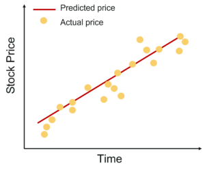
Let’s assume that you want to predict the price of a stock over a period of time. For such problems, you can make use of linear regression by studying the relationship between the dependent variable which is the stock price and the independent variable which is the time.
Predict Stock price – Linear Regression In R – Edureka
In our case, the stock price is the dependent variable, since the price of a stock depends and varies over time. And take note that the value of a stock is always a continuous quantity.
On the other hand, time is the independent variable that can be either continuous or discrete. And this independent variable is used to decide the value of the dependent variable.
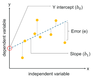
The first step in linear regression is to draw out a relationship between our dependent variable and independent variable by using a best fitting linear line.
Linear Regression In R – Edureka
We call it “Linear” regression, because both the variables vary linearly. Which means that, while plotting the relationship between two variables, we’ll get more of a straight line instead of curves.
Now let’s discuss the math behind linear regression.
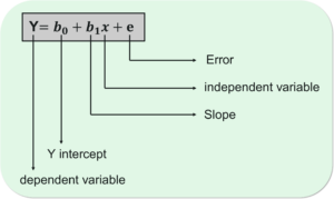
The below equation is used to draw out a relationship between the independent variable (X) and the dependent variable (Y). We all know the equation for a linear line in math is y=mx + c, so the linear regression equation is represented along the same equation:
 Linear Regression Model – Linear Regression In R – Edureka
Now that you have a good understanding of Linear Regression, let’s gets started with the implementation.
A lot of people have this question in mind, What does the R stand for in Linear Regression?
The answer is, R is basically an open-source programming and statistical language used for data analysis, data manipulation and data visualization. It is a multi-purpose programming language popularly used in the field of Machine Learning, Artificial Intelligence and Data Science.
Data Set Description:
In order to understand how linear regression model works, we’ll be using a simple data set containing the systolic blood pressure level for 30 people of different ages.
Problem Statement:
To build a linear regression model that can be used to predict the blood pressure of a person by establishing a statistically significant linear relationship with the corresponding age. We’ll be creating a Linear Regression model that will study the relationship between the blood pressure level and the corresponding age of a person.
Let’s take a look at the first 5-6 observations of our data set:
head(trainingSet)
  age y
1 39 144
2 47 220
3 45 138
4 47 145
5 65 162
6 46 142
The first step in building a regression model is to graphically understand our data. We need to understand the relationship between the independent and dependent variable by visualizing the data. We can make use of various plots such as Box plot, scatter plot and so on:
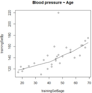
Scatter plot is a graphical representation used to plot data points via the x-axis and y-axis. The main purpose of a scatter plot is to represent the relationship between the dependent and the independent variable or the correlation between them.
scatter.smooth(x=trainingSet$age, y=trainingSet$y, main="Blood pressure ~ Age") # scatterplot
Scatter Plot – Linear Regression In R – Edureka
In the above illustration, the scatter plot shows a linear, positive correlation between the ‘age’ and ‘blood_pressure’ variables.
This shows that the relation between the response (dependent) and the predictor (independent) variable is linear, which is one of the fundamentals of a linear regression model.
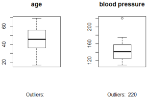
A box plot is mainly used in explanatory data analysis. A box plot represents the distribution of the data and its variability. The box plot contains the upper and lower quartiles, so the box basically spans the Inter-Quartile Range (IQR).
One of the main reasons why box plots are used is to detect outliers in the data. Since the box plot spans the IQR, it detects the data points that lie outside this range. These data points are known as outliers.
# Divide the graph area in 2 columns
par(mfrow = c(1, 2))
# Boxplot for X
boxplot(trainingSet$age, main='age', sub=paste('Outliers: ', boxplot.stats(trainingSet$x)$out))
# Boxplot for Y
boxplot(trainingSet$y, main='blood pressure', sub=paste('Outliers: ', boxplot.stats(trainingSet$y)$out))
Box Plot – Linear Regression In R – Edureka
The next significant measurement in Linear regression is Correlation.
Correlation is a statistical measure that shows the extent to which two or more variables vary together. There are two types of correlations:
If the value of the correlation between the dependent and independent variables is closer to zero, it indicates a weak relationship between them. The value of correlation is very important because it suggests if the dependent variable really varies based on the independent variable.
A correlation in the range of (-0.2 to 0.2) indicates a weak relationship between the response and predictor variable and hence suggests that the dependent variable does not essentially vary with respect to the independent variable. In such situations, it is considered wise to look for better predictor variables.
# Finding correlation
cor(trainingSet$age, trainingSet$y)
[1] 0.6575673
After studying the relation and calculating the correlation between the dependent and independent variable, its now time to build the linear regression model.
R comes with a predefined function for building a Linear Regression model. This function is known as the lm() function. The syntax for the lm() function is as follows:
lm(formula, data)
Let’s understand the two parameters:
# Fitting Simple Linear regression
regressor = lm(formula = y ~ age, data = trainingSet)
print(regressor)

Call:
lm(formula = y ~ age, data = trainingSet)

Coefficients:
(Intercept)    age
98.7147     0.9709
The above illustration shows our linear regression model along with the Coefficients. There are 2 parameters in the coefficient section:
These coefficients also known as beta coefficients are used to compute the value of the response variable (blood pressure).
The formula used here is:
Blood_pressure = Intercept + (b1 * age)
So far, we built the linear regression model and also computed the formula needed to calculate the blood pressure, given the age of a person. So, what next?
Our next step is to check the efficiency of our model. We need to recognize whether this model is statistically strong enough to make predictions.
In order to make sure the model is efficient, let’s take a look at the summary of the model:
summary(regressor)

Call:
lm(formula = y ~ age, data = trainingSet)

Residuals:
Min 1Q Median 3Q Max
-21.724 -6.994 -0.520 2.931 75.654

Coefficients:
            Estimate Std. Error t value Pr(>|t|)
(Intercept) 98.7147    10.0005   9.871  1.28e-10 ***
age         0.9709     0.2102    4.618  7.87e-05 ***
---
Signif. codes: 0 ‘***’ 0.001 ‘**’ 0.01 ‘*’ 0.05 ‘.’ 0.1 ‘ ’ 1

Residual standard error: 17.31 on 28 degrees of freedom
Multiple R-squared: 0.4324, Adjusted R-squared: 0.4121
F-statistic: 21.33 on 1 and 28 DF, p-value: 7.867e-05
The above summary tells us a couple of things:
Pay close attention to the p-value of the coefficients, (1.28e-10 and 7.87e-05)
In simple terms, p-value indicates how strong your regression model is. p-value is a very important measurement when it comes to ensuring the significance of the model. A linear model is said to be statistically significant only when both the p-Values are less than the pre-determined statistical significance level, which is ideally 0.05. The p-value for each coefficient is represented as a probability Pr(>|t|).
Before we discuss the Pr(>|t|), let’s discuss another important concept related to the p-value, which is the null and alternate hypothesis
In the summary of the model, notice another important parameter called the t-value. A larger t-value suggests that the alternate hypothesis is true and that the coefficients are not equal to zero by pure luck.
Pr(>|t|) is basically, the probability that, the obtained t-value is higher than the observed value when the Null Hypothesis holds true. In short, if the value of Pr(>|t|) is below 0.05, the coefficients are essential in the computation of the linear regression model, but if the Pr(>|t|) is high, the coefficients are not essential.
In our case,
The smaller the p-value of a variable, the more significant it is in predicting the value of the response variable. The stars corresponding to the p values indicate the significance of that respective variable. Since in our model, both the p values have a 3 star, this indicates that both the variables are extremely significant in predicting the dependent variable (Y).
R-squared is a statistical measure that represents the extent to which the predictor variables (X) explain the variation of the response variable (Y). For example, if R-square is 0.7, this shows that 70% of the variation in the response variable is explained by the predictor variables. Therefore, the higher the R squared, the more significant is the predictor variable.
Generally, R-square is used when there is only one predictor variable, but what if there are multiple predictor variables?
The problem with R-squared is that it will either remain the same or increase with the addition of more variables, even if they do not have any association with the output variables.
This is where Adjusted R square comes into the picture. Adjusted R-square restricts you from adding variables which do not improve the performance of your regression model. So, if you are building a regression model using multiple predictor variables, it is always recommended that you measure the Adjusted R-squared in order to detect the effectiveness of the model.
As mentioned earlier, residual is used to check the efficiency of the model by calculating the difference between the actual values and the predicted values and when the Residual Standard Error (RSE) is calculated as zero (this is highly unlikely in real-world problems) then the model fits the data perfectly. RSE is mainly used to check the model accuracy, the lower the RSE, the more accurate are the predictions made by the model.
The F-statistic is a statistical measure used to judge whether at least one independent variable has a non-zero coefficient. A high F-statistic value leads to a statistically accepted p-value (i.e., p < 0.05).
In our case, the F-statistic value is 21.33 which leads to a p-value of 7.867e-05, which is highly significant.
The statistical measures that I discussed above are very important when it comes to choosing an effective linear regression model. Only if the model is statistically significant, it can be used for predicting the dependent variable.
Now comes the interesting part. After checking the effectiveness of our model, lets now test our model on a separate, testing data set.
So, I’ve already created a separate testing data frame, I’ll be using this data set to test the model.
Step 1: Import the test data set
# Importing test data
testSet = read.csv('/Users/zulaikha/Desktop/test.csv')
Step 2: Use the linear regression model that you built earlier, to predict the response variable (blood pressure) on the test data
# Predicting the test results
regressor = lm(formula = y ~ age, data = trainingSet)
y_pred = predict(regressor, newdata = testSet)
Step 3: Evaluate the summary of the model
summary(regressor)

Call:
lm(formula = y ~ age, data = trainingSet)

Residuals:
Min 1Q Median 3Q Max
-21.724 -6.994 -0.520 2.931 75.654

Coefficients:
            Estimate Std. Error t value Pr(>|t|)
(Intercept) 98.7147   10.0005    9.871   1.28e-10 ***
age         0.9709    0.2102     4.618   7.87e-05 ***
---
Signif. codes: 0 ‘***’ 0.001 ‘**’ 0.01 ‘*’ 0.05 ‘.’ 0.1 ‘ ’ 1

Residual standard error: 17.31 on 28 degrees of freedom
Multiple R-squared: 0.4324, Adjusted R-squared: 0.4121
F-statistic: 21.33 on 1 and 28 DF, p-value: 7.867e-05
In the above illustration, the model p-value and independent variable’s p-value are less than the pre-determined standard significance level (0.05). Thus, we can conclude that our model is statistically significant.
Take note of the R-Sq and Adj R-Sq, they are comparatively similar to the original model that was created on the training data.
Step 4: Calculate prediction accuracy
The accuracy can be tested by comparing the actual values and the predicted values.
#Finding accuracy actuals_preds <- data.frame(cbind(actuals=testSet$y, predicted=y_pred)) correlation_accuracy <- cor(actuals_preds) head(actuals_preds) actuals predicted 1 144 136.5787 2 220 144.3456 3 138 142.4039 4 145 144.3456 5 162 161.8213 6 142 143.3748
In the above output, you can see that the predicted and actual values are not very far apart. In order to improve the accuracy, we can train the model on a bigger data set and try to use other predictor variables.
So, that was all about building a linear regression model in R from scratch.
Now that you know how Linear Regression works, I’m sure you’re curious to learn more about the various Machine learning algorithms. Here’s a list of blogs that covers the different types of Machine Learning algorithms in depth
With this, we come to the end of this Linear Regression In R blog. I hope you found this blog informative.
Stay tuned for more blogs on the trending technologies.
To get in-depth knowledge of the different machine learning algorithms along with its various applications, you can enroll here for live online training with 24/7 support and lifetime access.
Got a question for us? Mention them in the comments section of this ‘Linear Regression In R’ blog.
 Thank you for registering Join Edureka Meetup community for 100+ Free Webinars each month JOIN MEETUP GROUP
edureka.co