Understanding Cardinality of Relationships in Power BI: A Complete Guide

The Cardinality Of Relationships in Power BI plays an important role in defining the relationships between tables as part of the data modeling process. Proper data interpretation is made feasible with performance optimization, as well as highly accurate and efficient reports. Therefore, being well-versed in cardinality has been proven to facilitate the building of reliable models and significantly improve reporting efficiency.

In Power BI, the term “cardinality” describes the type of relationship between two tables according to how many related rows each table has. It specifies the relationships between rows in one table and rows in another. A key idea for specifying table relationships in any data model is cardinality.

What are Power BI Model Relationships?

Power BI model relationships are the connections between different tables in your database. They define how those tables are connected to and interact with one another. They will help you combine and analyze your data and give you precise calculations and visuals.

Now we will dive into the foundation of how data tables connect and interact within your Power BI model.

Power BI Model Relationships – Relationship Purpose

Filters applied to one model table’s column are propagated to another model table via a model relationship. As long as there is a relationship path to follow—which may include propagation to several tables—filters will continue to spread.

Relationship paths are deterministic, meaning filters propagate consistently and without chance. However, model calculations that use specific DAX functions can disable relationships or change the filter context.  

Next, dive into cardinality and its role in defining table connections.

What is the Cardinality of the relationship?

In Power BI, the term “cardinality” describes the type of relationship between two tables according to how many related rows each table has. It specifies the relationships between rows in one table and rows in another. A key idea for specifying table relationships in any data model is cardinality.

A cardinality type defines each model relationship. The data properties of the “from” and “to” related columns are represented by the four cardinality-type options. Whereas the “many” side indicates that the column may contain duplicate values, the “one” side suggests that the column contains unique values. 

Types of Cardinality

• • • One-to-Many (and Many-to-One) Cardinality
    • One-to-Many Cardinality (1:*)
    • Many-to-Many (:) Cardinality
    • Many-to-One (*:1) Cardinality

In Power BI Desktop, the cardinality type is automatically detected and set by the designer when you create a relationship. To determine which columns contain unique values, Power BI Desktop runs queries against the model. It sends profiling queries to the data source for DirectQuery models and uses internal storage statistics for import models. However, Power BI Desktop occasionally makes mistakes. When tables have not yet been loaded with data or when columns that you anticipate to have duplicate values now contain unique values, it may make a mistake. As long as any “one” side columns have unique values or the table hasn’t been loaded with rows of data, you can change the cardinality type in either scenario. 

• One-to-Many (and Many-to-One) Cardinality

Every row in the first table has a one-to-one relationship with exactly one row in the second table. When every record in both tables has a unique match, this kind of relationship—which is comparatively uncommon—is employed.

Use Case: 1:1 relationships are most helpful when dividing a large

• One-to-Many Cardinality (1:*)

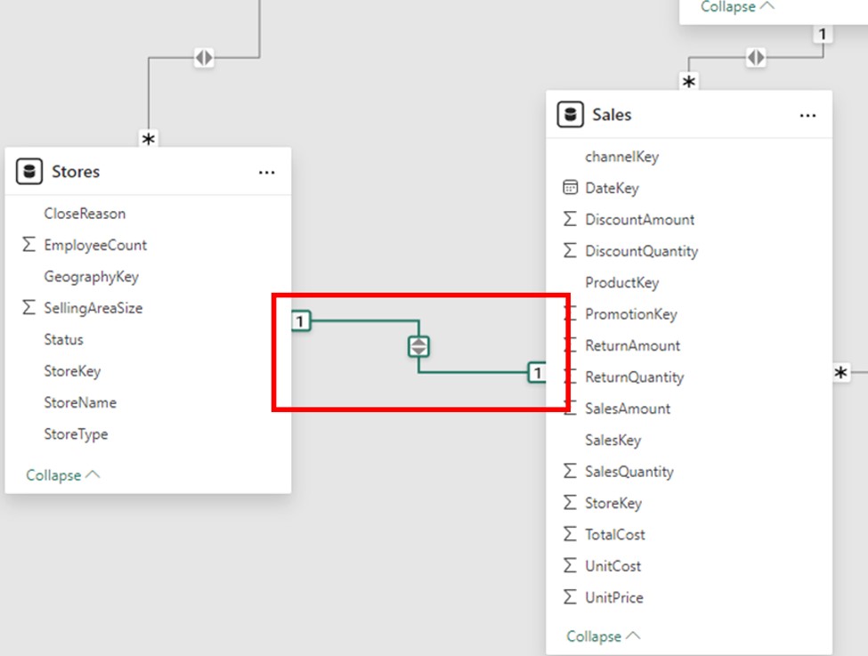
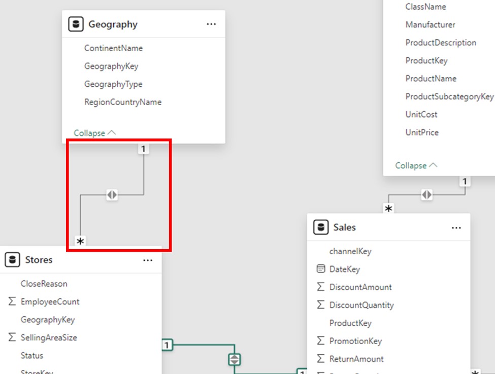
The most prevalent kind of cardinality in Power BI is one-to-many. In this relationship, a single row in one table may correlate to several rows in another table. Usually, the “one” side is referred to as the “lookup” table, and the “many” side is called the “fact” table.

Use Case: 1:  Cardinality is necessary for creating data models that aggregate data, such as those used to monitor product sales, client interactions, or order histories. 

• Many-to-Many (:) Cardinality

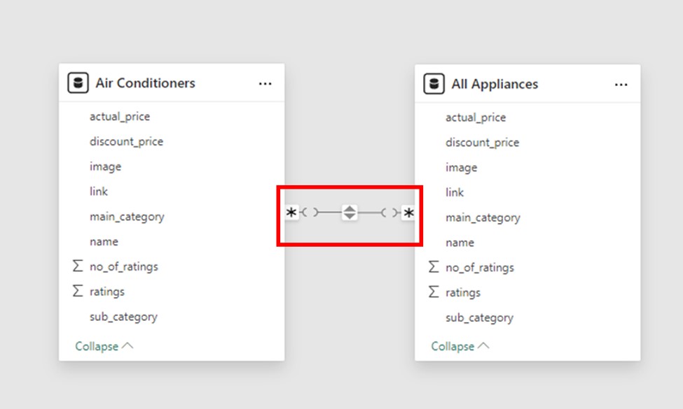
When both tables have non-unique values in the corresponding columns that are part of the relationship, the Many-to-Many cardinality is employed. Because it permits multiple matches between rows in both tables, this kind of cardinality can be challenging. To make modeling complex data scenarios easier and eliminate the need for bridge tables, Power BI introduced support for relationships.

Use Case: Many-to-many relationships are particularly helpful in situations involving shared entities.

• Many-to-One (*:1) Cardinality

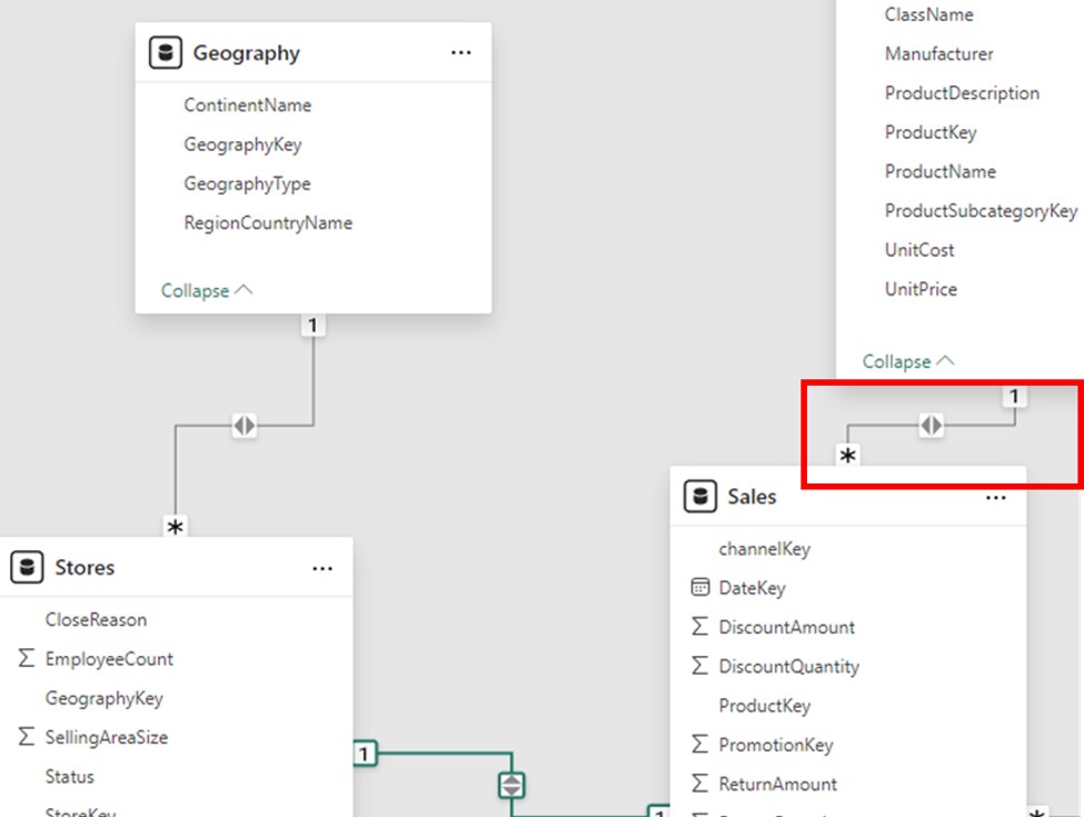
In essence, a Many-to-One relationship is the opposite of a One-to-Many relationship. In this case, a single row in the second table can map to numerous rows in the first table. When building relationships, Power BI automatically recognizes this situation, particularly when modeling data that has been imported from other systems.

Use Case: This cardinality is the norm for data summarization and filtering.

Moving forward, we’ll discuss how cross-filtering influences data flow.

Cross Filter Direction

In Power BI, each model relationship has a cross-filter direction that dictates how filters move between tables. The cardinality type of the relationship determines the cross-filter options.

• Direction of a Single Cross Filter: Filters move in a single direction, either from the “one” side to the “many” side or the other way around.
• Both Cross-Filter Directions: A bi-directional relationship is created by filters that propagate in both directions. 

The cross-filter direction is always from the “one” side for one-to-many relationships, but it can also be set to be bidirectional. The cross-filter direction is always active in both tables for one-to-one relationships. The cross-filter direction can be set from either table or both in many-to-many relationships.

When both cross-filter directions are enabled, an extra feature that applies bidirectional filtering when Power BI enforces row-level security (RLS) rules is available. Bidirectional relationships, however, could have a detrimental effect on performance and result in unclear filter propagation paths. A resolution is required if Power BI Desktop fails to commit to the relationship change or permits the definition of unclear relationship paths between tables.

Bi-directional filtering should only be used when necessary, and the possible performance effects should be carefully considered. By using the CROSS FILTER DAX function in model calculations, Power BI users can change the relationship cross-filter direction, including turning off filter propagation. 

After that, learn why activating relationships ensures accurate reporting.

Make This Relationship Active

There can only be one active filter propagation path between two tables per model in Power BI. Other relationship paths could be added, though, but they would need to be marked as dormant. The USERELATIONSHIP DAX function allows you to activate inactive relationships while assessing a model calculation temporarily.

Since active relationships enable users to use your model effectively, it is ideal to define them whenever possible. When utilizing only active relationships, role-playing dimension tables should be replicated in the model.

However, in some situations, it might be appropriate to define one or more inactive relationships for a role-playing dimension table. When filtering by multiple roles at the same time is not necessary, this design may be taken into consideration. Users can perform custom filtering according to their needs by using the USERELATIONSHIP DAX function to activate a specific relationship for pertinent model calculations.

Now, let’s understand when to use this feature for better performance.

Assume Referential Integrity

Only one-to-many and one-to-one relationships between two DirectQuery storage mode tables that are part of the same source group are covered by the “Assume referential integrity” property. When there are no NULL values in the “many” side column, it can be enabled. Data is not imported into the model when using DirectQuery mode. Rather, the model’s structure is defined only by metadata. In order to retrieve real-time data, native queries are sent straight to the underlying data source when they are executed.

This property, when enabled, guarantees that native queries sent to the data source join the two tables using an INNER JOIN rather than an OUTER JOIN. Enabling this property generally improves query performance, though the amount of improvement varies depending on the data source.

Enabling this property is always advised when there is a database foreign key constraint between the two tables. Additionally, if you are confident in the data integrity, think about turning on the property even in situations where there isn’t a foreign key constraint. This could optimize query performance further.

 Next, we’ll look at DAX functions that utilize relationships for advanced calculations.

Relevant DAX Functions

In Power BI, several DAX functions are crucial for managing model relationships. Below is a synopsis of each function:

• RELATED: This function retrieves the value from the “one” side of a relationship, making it useful for cross-table computations assessed in row context.
• RELATED TABLE: This function pulls a table of rows from a relationship’s “many” side.
• USERELATIONSHIP: This feature enables computations to make use of inactive relationships, which is especially helpful when working with dimension tables in role-playing or clearing up ambiguity in filter paths.
• CROSSFILTER: This feature allows you to change or ignore model relationships during certain calculations by changing the relationship cross-filter direction (to one or both) or turning off filter propagation (none).
• COMBINE VALUES: Enables multi-column relationships in DirectQuery models within the same source group by joining several text strings into one.
• TREATS: Allows the establishment of virtual relationships during particular computations by applying the results of a table expression as filters to columns from an unrelated table.

The parent and child functions, a family of related functions that help create calculated columns to naturalize a parent-child hierarchy, make the creation of fixed-level hierarchies possible.

Continuing, explore how Power BI evaluates relationships for data accuracy.

Relationship Evaluation

Based on the cardinality type and the data source of the related tables, model relationships are automatically classified as either regular or limited from an evaluation perspective. Understanding the evaluation type is crucial since it can affect data integrity and performance.

First, some modeling theory is required to comprehend relationship evaluations. All of the data in an import or DirectQuery model comes from the source database or the Vertipaq cache, which enables Power BI to identify whether a relationship has a “one” side.

Each source, however, constitutes a source group in a composite model, which can incorporate tables with various storage modes (import, DirectQuery, or dual) or multiple DirectQuery sources. There are two types of model relationships in a composite model: intra-source groups and inter/cross-source groups. Whereas an inter/cross-source group relationship links tables from various source groups together, an intra-source group relationship links tables within the same source group. Relationships in import or DirectQuery models are always regarded as intra-source group relationships, so keep that in mind.

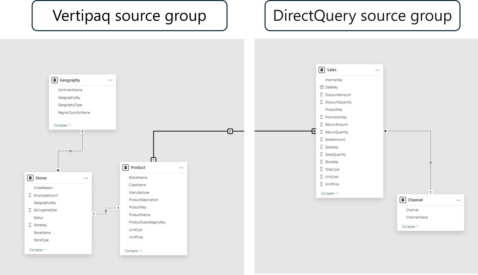Take, for example, a composite model that has two source groups: one with three tables from Vertipaq and one with two tables from DirectQuery. In this instance, a table in the Vertipaq source group is related to another table via a cross-source group relationship.

Now, focus on standard relationships and their typical use cases.

Regular Relationships

When the query engine can identify the “one” side of a relationship, it is regular. The unique values in the “one” side column have been confirmed. Every one-to-many relationship within the source group is a regular relationship.

The following example shows two regular relationships as R. Two examples of relationships are the one-to-many relationships found in the DirectQuery source and the Vertipaq source group.

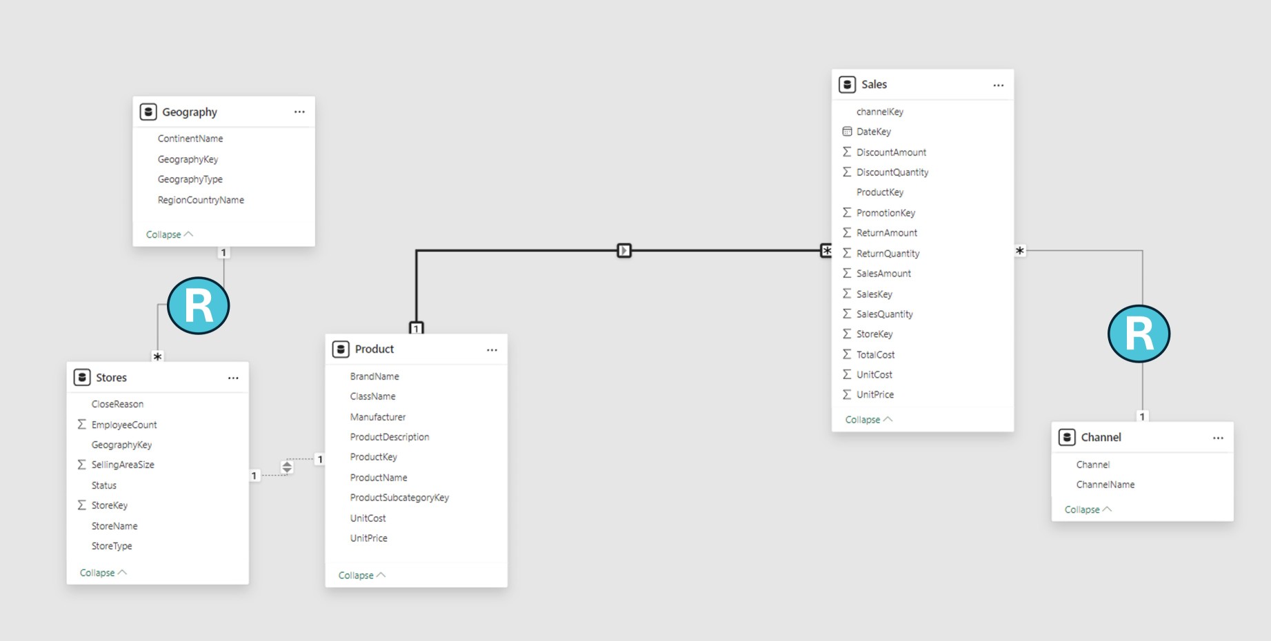At data refresh time, Power BI generates a data structure for every regular relationship in import models, where all data is kept in the Vertipaq cache. To speed up joining tables at query time, the data structures are made up of indexed mappings of all column-to-column values.

Regular relationships allow table expansion to occur at query time. By adding the base table’s native columns and then expanding into related tables, table expansion creates a virtual table. Table expansion for DirectQuery tables is done in the native query that is sent to the source database (provided that the Assume referential integrity property is not enabled); for import tables, it is done in the query engine. The query engine then acts upon the expanded table, applying filters and grouping by the values in the expanded table columns.

 Afterward, we’ll cover limited relationships and their specific applications.

Limited relationships

A model relationship is limited when there’s no guaranteed “one” side. A limited relationship can happen for two reasons:

Even though one or both columns have unique values, the relationship employs a many-to-many cardinality type.
There is a cross-source group relationship, which is only possible for composite models.

The following example shows two limited relationships, L: the one-to-many cross-source group relationship and the many-to-many relationship found in the Vertipaq source group.

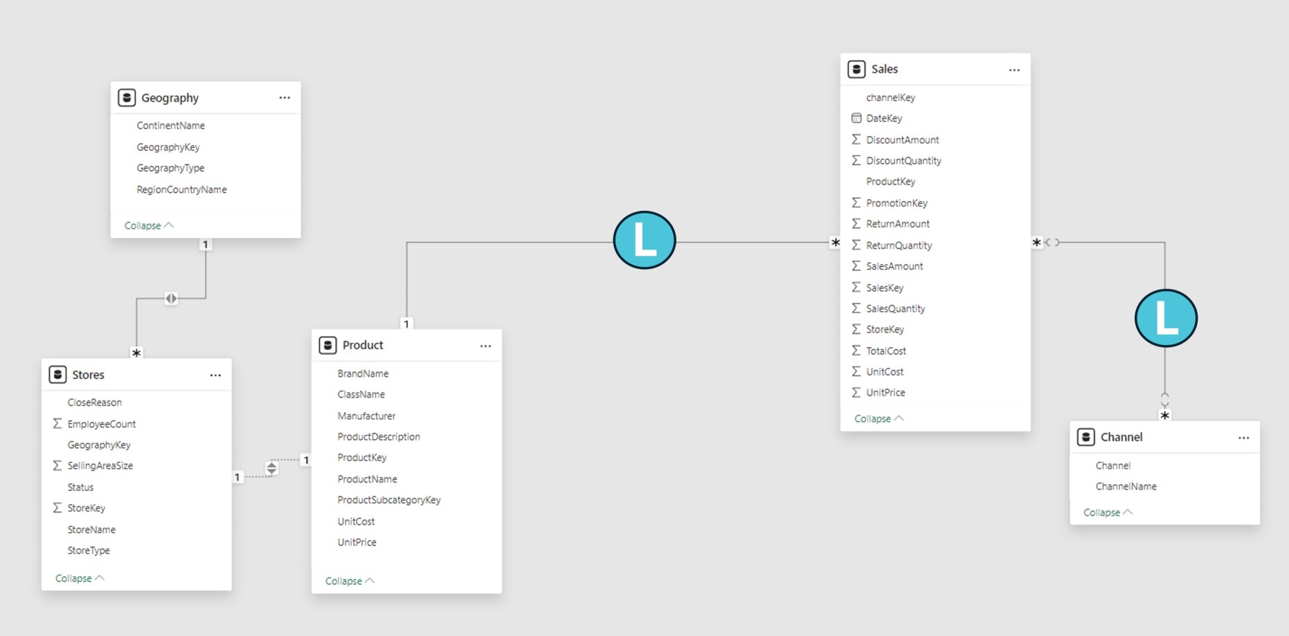Data structures are never made for limited relationships in import models. Table joins are then resolved at query time by Power BI.

For limited relationships, there is never any table expansion. Blank virtual rows are not added to make up for referential integrity violations because table joins are accomplished using INNER JOIN semantics.

There are other restrictions related to limited relationships:

• The RELATED DAX function can’t be used to retrieve the “one” side column values.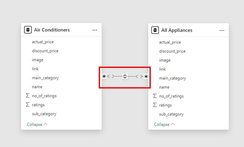
• Enforcing RLS has topology restrictions.

Next, discover how to address multiple paths to avoid data conflicts.

Resolve Relationship Path Ambiguity

Bi-directional relationships have the potential to introduce multiple filter propagation paths between model tables, which can be confusing. Power BI selects the filter propagation path based on its priority and weight when assessing ambiguity.

Priority
To resolve relationship path ambiguity, Power BI employs a set of rules defined by priority tiers. The first rule match determines Power BI’s course. Each of the following rules explains the flow of filters from a source table to a target table.

• Priority is given to a path with one-to-many relationships.
• A path with one-to-many or many-to-many relationships is taken into consideration if there isn’t a one-to-many path.
• A path with many-to-one relationships is then assessed.
• If no obvious path has been identified yet, a combination of one-to-many relationships from the source table to an intermediate table and many-to-one relationships from the intermediate table to the target table is taken into consideration.
• In a similar vein, relationships between the source table and an intermediate table that are one-to-many or many-to-many, followed by many-to-one or many-to-many relationships between the intermediate table and the target table, are investigated.
• As a last resort, all other options are considered.

Weight
Every connection on a path has a weight. Unless the USERELATIONSHIP function is used, all relationship weights are set to equal by default. All relationship weights along the path add up to the path weight. Power BI resolves ambiguity between multiple paths in the same priority tier by using the path weights. It will select the path with the higher weight rather than the one with a lower priority. The weight is independent of the number of relationships in the path.

The USERELATIONSHIP function allows you to change a relationship’s weight. The call to this function’s nesting level determines the weight, with the innermost call carrying the most weight.

Consider the following example. The Product Sales measure assigns a higher weight to the relationship between Sales[ProductID] and Product[ProductID], followed by the relationship between Inventory[ProductID] and Product[ProductID].

Product Sales =

CALCULATE(

CALCULATE(

SUM(Sales[SalesAmount]),

USERELATIONSHIP(Sales[ProductID], Product[ProductID])

),

USERELATIONSHIP(Inventory[ProductID], Product[ProductID])

)

Finally, we’ll discuss optimizing relationships for better model efficiency.

Preference for performance

Filter propagation performance is ranked from fastest to slowest in the following list:

• The fastest filter propagation speed is found in one-to-many relationships within the same source group.
• In terms of performance, many-to-many relationships with at least one bidirectional relationship accomplished through an intermediary table come next.
• The filter propagation speed of many-to-many cardinality relationships is moderate.
• The slowest filter propagation performance is found in cross-source group relationships.

To wrap up, summarize the key concepts for mastering Power BI relationships.

Conclusion

Cardinality in Power BI refers to how the tables are related, e.g., one-to-one, one-to-many, or many-to-many. It ensures connecting the data correctly and performing calculations without error. It also makes reports’ performance efficient as it prevents errors concerning cardinality.

Lastly, address common queries to solidify your understanding of these concepts.

FAQs

1. What does cardinality mean in relationships in Power BI?

Cardinality refers to how two tables have a relationship, such that they are either one too many, many to one, many to many, or one-to-one.

2. How do I select the appropriate cardinality for my tables?

Analyze your data; use one-to-many for primary and foreign keys or many-to-many when it does not have a unique key.

3. What are some of the problems brought about by an incorrect cardinality?

Incorrect cardinality creates duplicate data, incorrect aggregation, and many performance issues when reading the report.

4. Can the cardinality of a relationship be changed?

Yes, you can edit the relationship in Model View and adjust your cardinality according to the needs of your data.

5. When is a many-to-many relationship appropriate?

Many-to-many tables are appropriate when examining non-aggregation among them where no unique keys exist in both tables.

Also Please Check out Edureka’s Power BI Interview question and Answer which is given Below:

https://www.edureka.co/blog/interview-questions/power-bi-interview-questions/  

This would effectively end the discussion about blog post cardinality in Power BI, which undoubtedly defines relationships within tables. The post also included hints about how cardinality affects data accuracy, model performance, and reporting efficiency. Mastering it ensures that you can create high-quality, effective Power BI dashboards tailored to your specific requirements.

If you are interested in advancing your skills and your career prospects as a Power BI developer, then you should explore the latest courses and Training programs. We recommend you take up the Microsoft Power BI Certification Training: PwC Academy offered by Edureka. The Edureka’s Power BI certification course by PwC offers dual certification in business intelligence. The training is live instructor-led and provides hands-on experience in real-time projects. It prepares you for the official PL-300 exam and offers simulated real-world scenarios.

Do you have any questions or need further information? Feel free to leave a comment below, and we’ll respond as soon as possible!