Capsule Neural Networks – Set of Nested Neural Layers

Capsule Networks:

What is Capsule Networks? It is basically, a network of set of nested neural layers. 

I would recommend you to go through the below blogs as well:

• Single Layer Perceptron
• Neural Network Tutorial
• Backpropagation

I am assuming that, you guys know Convolutional Neural Networks (CNN). Here, I will be giving you a small introduction on the same, so that I can discuss the limitations of CNNs.

You can also refer the below video on Convolutional Neural Network.

Convolutional layer: When we use Feedforward Neural Networks (Multi Layer Perceptron) for image classification, there are many challenges with it. The most frustrating challenge is that, it introduces a lot of parameters, consider the video tutorial on CNN.

To overcome this challenge Convolution Layer was introduced. it is assumed that, pixels that are spatially closer together will “cooperate” on forming a particular feature of interest much more than ones on opposite corners of the image. Also, if a particular (smaller) feature is found to be of great importance when defining an image’s label, it will be equally important, if this feature was found anywhere within the image, regardless of location.

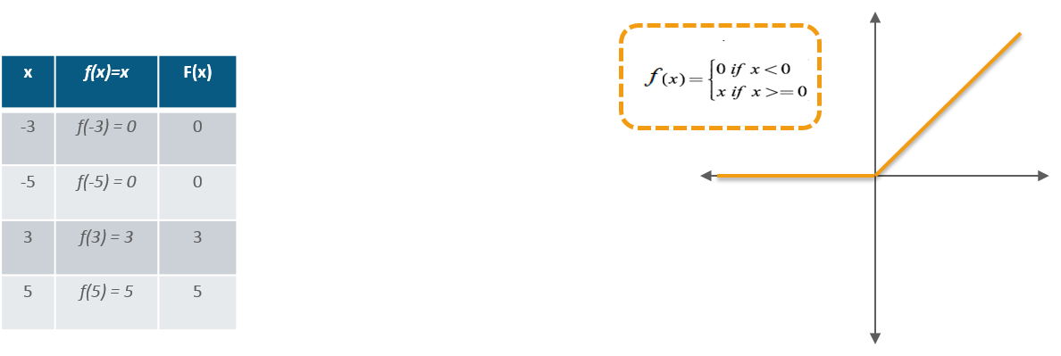
ReLU Layer: Rectified Linear Unit (ReLU) transform function only activates a node if the input is above a certain quantity, while the input is below zero, the output is zero, but when the input rises above a certain threshold, it has a linear relationship with the dependent variable. 

• In this layer we remove every negative values from the filtered images and replaces it with zero’s
• This is done to avoid the values from summing up to zero

Pooling Layer: This is used to perform downsampling, which consumes small and (usually) disjoint chunks of the image and aggregates them into a single value. There are several possible schemes for the aggregation – the most popular being Max-Pooling, where the maximum pixel value within each chunk is taken. It makes the network invariant to small transformations, distortions and translations in the input image (a small distortion in input will not change the output of Pooling – since we take the maximum / average value in a local neighborhood).

Fully Connected Layer: This layer will compute the class scores, where each of the numbers correspond to a class score. As with ordinary Neural Networks and as the name implies, each neuron in this layer will be connected to all the neurons in the previous volume. In a nutshell, it performs the final classification.

Note: Training of this model is done by Backpropagation, so you can check this separate blog on Backpropagation.

In this way, ConvNets transform the original image layer by layer from the original pixel values to the final class scores.

This was a very short introduction to Convolutional Neural Networks, I would still recommend you to have a look at the CNN video that I have embedded in this post.

In this Capsule Networks blog, I will now discuss few limitations of Convolutional Neural Networks

Limitations Of Convolutional Neural Networks:

Well, let me explain this with an analogy.

Suppose there is a human, whose eyes can detect the features of various images. Let us consider the face of a human as an example. So, this unfortunate guy can identify various features such as, eyes, nose etc. but, is unable to identify the spatial relationships among features (perspective, size, orientation). For example, the following picture may fool that guy in classifying it as a good sketch of a human face.

This is the problem with Convolutional Neural Networks as well. CNN is good at detecting features, but will wrongly activate the neuron for face detection. This is because it is less effective at exploring the spatial relationships among features.

A simple CNN model can extract the features for nose, eyes and mouth correctly but will wrongly activate the neuron for the face detection. Without realizing the mis-match in spatial orientation and size, the activation for the face detection will be too high.

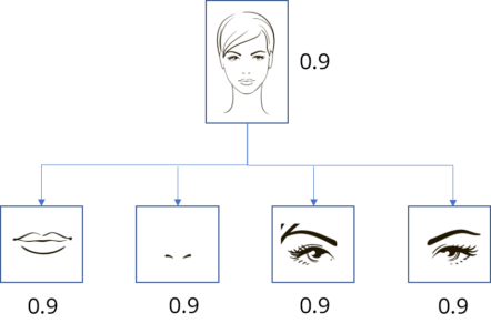
Well, this limitation is because of the Max Pooling layer.

The max pooling in a CNN handles translational variance. Even a feature is slightly moved, if it is still within the pooling window, it can still be detected. Nevertheless, this approach keeps only the max feature (the most dominating) and throws away the others.

So, the face picture shown above will be classified as a normal face. Pooling layer also adds this type of invariance.

This was never the intention of the pooling layer. What the pooling was supposed to do is to introduce positional, orientational, proportional invariances.

In reality, this pooling layer adds all sorts of positional invariance. As you can see in the above diagram as well, it leads to the dilemma of detecting the face correctly.

Let’s see what is the solution proposed by Geoffrey Hinton.

How to Solve This Problem?

Now, we imagine that each neuron contains the likelihood as well as properties of the features. For example, it outputs a vector containing [likelihood, orientation, size]. With this spatial information, we can detect the in-consistence in the orientation and size among the nose, eyes and ear features and therefore output a much lower activation for the face detection.

In the paper released by Geoffrey Hinton, these types of neurons are called capsules. These capsules output a vector instead of a single scaler value.

Let me put some lights on what are Capsule Networks.

What are Capsule Networks?

Capsule is basically, a set of nested neural layers. The state of the neurons inside a capsule captures the various properties like – pose (position, size, orientation), deformation, velocity, texture etc, of one entity inside an image.

Instead of capturing a feature with a specific variant, a capsule is trained to capture the likeliness of a feature and its variant. So, the purpose of the capsule is not only to detect a feature but, also to train the model to learn the variant.

Such that the same capsule can detect the same object class with different orientations (for example, rotate clockwise):

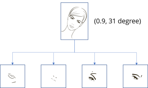
We can say it works on equivariance not invariance.

Invariance: is the detection of features regardless of the variants. For example, a nose-detection neuron detects a nose regardless of the orientation.

Equivariance: is the detection of objects that can transform to each other (for example, detecting faces with different orientations). Intuitively, the capsule network detects the face is rotated right 31° (equivariance) rather than realizes the face matched a variant that is rotated 31°. By forcing the model to learn the feature variant in a capsule, we may extrapolate possible variants more effectively with less training data. In additionally, we may reject adversaries more effectively.

A capsule outputs a vector to represent the existence of the entity. The orientation of the vector represents the properties of the entity.

The vector is sent to all possible parents in the neural network. For each possible parent, a capsule can find a prediction vector. Prediction vector is calculated based on multiplying it’s own weight and a weight matrix. Whichever parent has the largest scalar prediction vector product, increases the capsule bond. Rest of the parents decrease their bond. This is called as Routing By Agreement.

This is definitely a better approach then max pooling, in which routing is based on the strongest feature detected in the lower layer.

After this there is a squashing function which is added. This is done to introduce non – linearity. This squashing function is applied to the vector output of each capsule.

Let me tell you now, how Capsule Networks work.

How Capsule Networks Work?

Let us take a step back. In a fully-connected network, the output of each neuron is the weighted sum of the inputs.

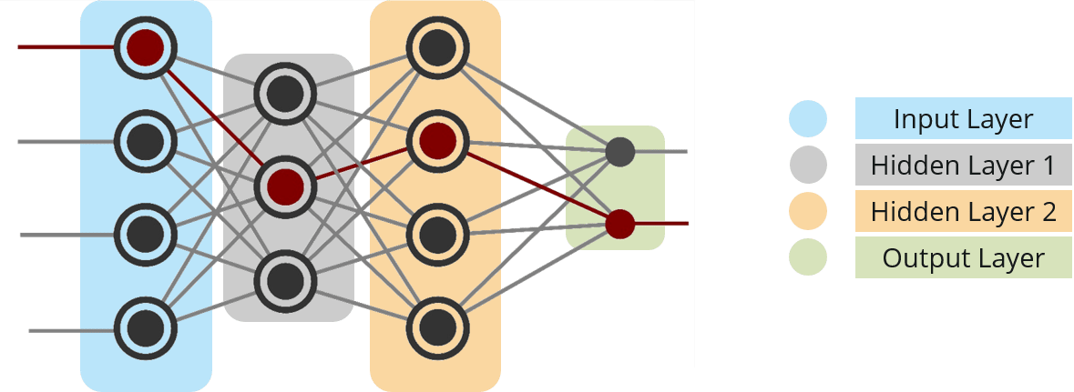
Now, let’s see what happens in Capsule Networks.

Capsule Neural Network:

Let us consider a Capsule Neural Network where ‘ui‘ is the activity vector for the capsule ‘i’ in the layer below.

Step – 1: Apply a transformation matrix Wij to the capsule output ui of the previous layer. For example, with a m×k matrix, we transform a k-D ui to a m-D u^j|i. ((m×k) × (k×1) = m×1).

It is the prediction (vote) from the capsule ‘i’ on the output of the capsule ‘j’ above. ‘vj‘ is the activity vector for the capsule ‘j’ in the layer above

Step – 2: Compute a weighted sum sj with weights cij. cij are the coupling coefficients. Sum of these coefficients is equal to one. It’s the actual parameter that works on the relationship of group of capsules that we talked earlier.

Step – 3: In Convolutional Neural Networks we used ReLU function. Here, we will apply a squashing function to scale the vector between 0 and unit length. It shrinks small vectors to zero and long vectors to unit vectors. Therefore the likelihood of each capsule is bounded between zero and one.

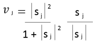
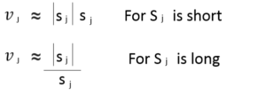
It is the prediction (vote) from the capsule ‘i’ on the output of the capsule ‘j’ above. If the activity vector has close similarity with the prediction vector, we conclude that capsule ‘i’ is highly related with the capsule ‘j’. (For example, the nose capsule is highly related to the face capsule.) Such similarity is measured using the scalar product of the prediction and activity vector. Therefore, the similarity takes into account on both likeliness and the feature properties. (instead of just likeliness in neurons).

Step – 4: Compute relevancy score ‘bij‘. It will be the dot product of the activity vector and the prediction vector. The coupling coefficients cij is computed as the softmax of bij:

The coupling coefficient cij is computed as the softmax of bij. 

This bij is updated iteratively in multiple iterations.

This is called as Routing By Agreement.

Below diagram is one example:

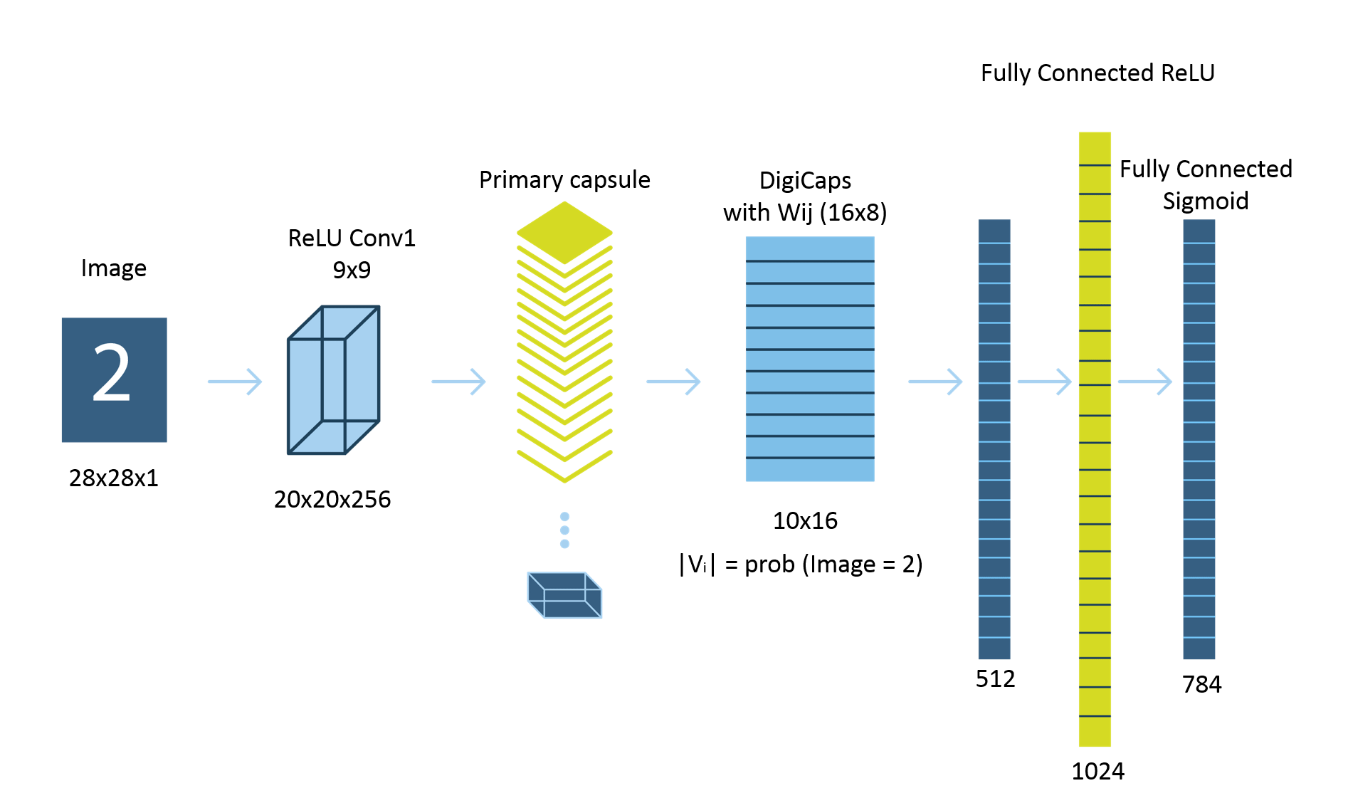
After this blog on Capsule Networks, I will be coming up with a blog on Capsule Neural Network implementation using TensorFlow.

Check out this NLP Course by Edureka to upgrade your AI skills to the next levelThe Edureka Deep Learning with TensorFlow Certification Training course helps learners become expert in training and optimizing basic and convolutional neural networks using real time projects and assignments along with concepts such as SoftMax function, Auto-encoder Neural Networks, Restricted Boltzmann Machine (RBM).

Got a question for us? Please mention it in the comments section and we will get back to you.